Adaptive Join

Introduction

The Adaptive Join operator is one of four operators that join data from two input streams into a single combined output stream. Unlike the three other join operators, Adaptive Join has not two but three inputs. Microsoft has not published any official naming for these inputs, but based on how the operator works they should be called (top to bottom in the graphical execution plan) build input, probe input, and inner input is at the bottom. The build input corresponds to the left input for the join; the probe and inner inputs are two alternative options to process the right input.

The Adaptive Join operator was added in SQL Server 2017 as an alternative to the other join operators: Nested Loops (ideal for joining a small data stream with a cheap input), Hash Match (most effective for joining large unsorted sets) and Merge Join (ideal for joining data streams that are sorted by the join key). It is intended to be used when there is no efficient way to fulfill the order requirement of the Merge Join, and the optimizer cannot reliably predict which of the remaining algorithms (Hash Match or Nested Loops) would perform best.

Because it has to be able to join the data using either the Nested Loops or the Hash Match algorithm, Adaptive Join suffers from the combined restrictions of these operators. As such, Adaptive Join supports only four logical join operations: inner join, left outer join (but not the probed version), left semi join, and left anti semi join;  it requires at least one equality-based join predicate, it uses lots of memory, and it is semi-blocking.

Visual appearance in execution plans

Depending on the tool being used, a Hash Match operator is displayed in a graphical execution plan as shown below:

SSMS and ADS (current versions)	Legacy SSMS	Plan Explorer	Paste The Plan

Algorithm

The best way to describe how Adaptive Join behaves is to see it as one top-level algorithm that guides the overall logic by invoking different lower-level algorithms where the actual operations are executed.

Top-level

The algorithm for the top-level logic of an Adaptive Join is as shown below:

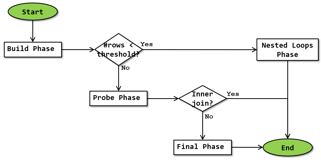
The operator starts by doing the same build phase that Hash Match does as its first phase. Once finished, the actual number of rows that was produced by the build input (and stored in the hash table) is compared to the Adaptive Threshold Rows property, to determine whether to continue with either the probe phase and optionally (depending on logical join type) the final phase, or to continue with the nested loops phase.

Build phase

The build phase of the Adaptive Join operator is exactly the same as the standard version of Hash Match’s build phase. The flowchart is repeated below:

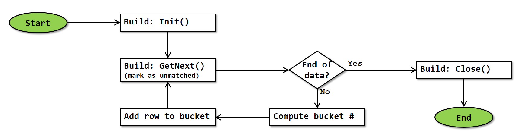
Note that, since Adaptive Join always starts in batch mode, this flowchart is actually a simplification. In reality, GetNext() requests and receives a full batch of rows from the build input. The operator then loops through the rows in that batch, computing the hash for each row and storing them in the hash table. More precise details of how batch mode works are at this time not known.

Probe phase

The probe phase occurs after the build phase, if the actual number of rows processed during the build phase is equal to or greater than the Adaptive Threshold Rows property. This means that the operator proceeds using the hash match algorithm. The flowchart for the probe phase of Adaptive Join is exactly the same as that of the probe phase of Hash Match, except that the logic for handling logical join types not supported by Adaptive Join has been removed. (Note: It is possible that Microsoft actually reuses the same code; in that case the logic for handling unsupported logical join types would still be executed)

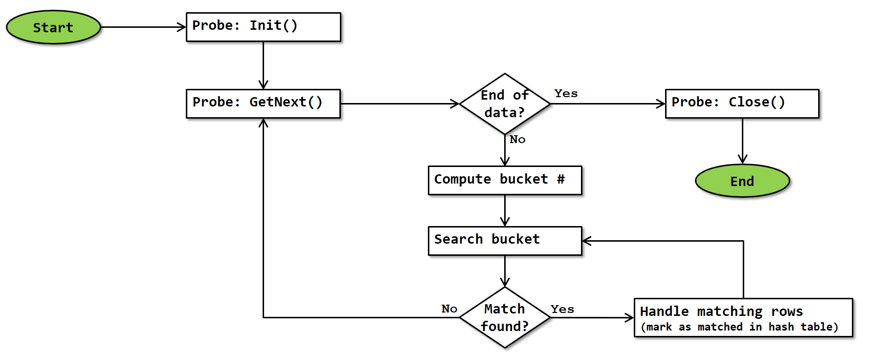
Note that, since the probe phase of Adaptive Join always runs in batch mode, this flowchart is actually a simplification. In reality, GetNext() requests and receives a full batch of rows. The operator then computes the hash for each of them, finds matches and adds them to the output batch. When an output batch is full, it is returned to the calling operator; the operation of Adaptive Join then waits until called again; at that point a new output batch is initialized and then the processing continues where it was. More precise details of how batch mode works are at this time not known.

Just as the probe phase of Hash Match, the algorithm has to check the key columns for exact match due to the risk of hash collision; and the bucket is always scanned completely because there may be more than one matching row in it. When a match is found, the row in the hash table is marked as “matched”; this is then later used to identify and handle unmarked rows. For logical join types inner join and left outer join, a row with the combined data is also added to the batch of rows to be returned to the calling operator.

Final phase

If the actual number of rows processed during the build phase is equal to or greater than the Adaptive Threshold Rows property, and the logical join type is Left Outer Join, Left Semi Join, or Left Anti Semi Join, then the probe phase is followed by a final phase. This phase performs the exact same logic as the normal final phase of a Hash Match operation, as shown in this flowchart:

Since rows in the hash table were marked as unmatched when they were added during the build phase, and those that were matched were then marked as matched during the probe phase, the algorithm can now go over all the rows in the hash table and verify which were matched and which were not. For a Left Outer Join or a Left Anti Semi Join, “Handle unmatched build row” returns the row whereas “Handle matched build row” does nothing; for a Left Semi Join this logic is reversed.

Since the final phase of Adaptive Join also always runs in batch mode, “returning a row” in the paragraph above does not mean returning a row and then passing control to the parent as it would in row mode; it adds the row to the output batch and continues. Control is only returned to the calling operator when the output batch is full; once the operator is called again a new output batch is initialized and processing continues where it was. More precise details of how batch mode works are at this time not known.

Nested Loops phase

The Nested Loops phase occurs after the build phase, if the actual number of rows processed during the build phase is less than the Adaptive Threshold Rows property. This means that the operator proceeds using the nested loops algorithm. A normal Nested Loops operator takes data for its outer loop from the top input of the operator; for an Adaptive Join that output has already been processed and is stored in the hash table, so that is where the output comes from in this case.

Other than reading the outer input data from the hash table instead of from a child operator, this flowchart is mostly identical to the flowchart for a Nested Loops operator. The main difference is that there is no need to test whether data returned from the inner input is a match, because the inner input of an Adaptive Join is always a dynamic inner input.

As always, the flowchart is a simplification because it doesn’t show that control is returned to the parent operator whenever a row is returned, and then execution doesn’t resume until the operator is called again. And, unlike the build, probe, and final phases, that actually happens as described here in the case of a nested loops phase, because this phase always runs in row mode.

Just as with a “normal” Nested Loops operator, the “handle matching rows” block will return the combination of the outer and inner row for an Inner Join or a Left Outer Join, or just the data from the outer input for a Left Semi Join. The “Handle unmatched outer row” block then is where the outer data is returned in the case of a Left Anti Semi Join.

Special considerations

Batch mode

The Adaptive Join operator can only be used in execution plans that use batch mode. As far as currently known, the operator itself has to execute in batch mode. In reality this means that it starts to execute in batch mode, however if the number of rows is below the threshold where it switches to the nested loops algorithm it will do that part of its work in row mode. (Batch mode will be described in detail at a later time).

Blocking

The Adaptive Join, like the Hash Match operator, can be considered to be “semi-blocking”. And like Hash Match, that is a simplification of reality.

The first phase, the build phase, always runs first, reads the entire build input, and stores it in memory. This phase is always blocking. After that, it depends on the logical join type, and on the number of rows.

Nested Loops

When the number of rows is below the threshold and the nested loops algorithm is chosen, then the second phase to run is the nested loops phase, which is streaming. Because this follows the blocking behavior of the build phase, that makes the actual behavior of the operator as a whole semi-blocking for this case.

Hash Match

If the number of rows is equal to or more than the threshold so that the hash match algorithm is used instead, then the probe phase comes second. For the logical join types Inner Join and Left Outer Join, this probe phase can start returning rows (in batches) as soon as matching data is found, so again this is a streaming behavior and the operator as a whole is semi-blocking.

However, for the logical join types Left Semi Join and Left Anti Semi Join, the probe phase merely marks data in the hash table as matched as probe rows are read; no data is returned at all until the final phase runs. So in those cases the behavior switches to fully blocking.

Memory usage

Since the Adaptive Join operator stores the entire build input in an in-memory hash table, it needs a large amount of memory to work with. The requested memory is computed when the execution plan is compiled and stored in the Memory Grant property of the execution plan. Since that property applies to the entire execution plan, it represents the (estimated) memory requirement of all operators in the execution plan – or at least all that need their memory concurrently.

The memory requirement of individual operators is not stored in the execution plan, though you can sometimes reverse engineer this from the Memory Grant of the plan as a whole and the Memory Fractions properties of the individual operators. This will be the subject of a future article.

No exact details are known for the memory grant computation of Adaptive Join. I assume that the same logic applies as for Hash Match, which means that not only the expected size (Estimated Number of Rows multiplied by Estimated Row Size) of the build input, but also (to some extent) the expected size of the probe input is taken into account.

Spilling

As described above, the memory grant is computed based on estimated cardinalities. If at runtime the actual cardinality (or the actual average row size) is much larger, the execution engine might run out of memory. In that case, the exact same spilling process happens as when a Hash Match operator runs out of memory. Please see the Hash Match page for a full description of this process.

Typically, spilling would only happen if the number of rows is much higher than the Adaptive Threshold Rows property. However, it is at least theoretically possible, when working with very large and expensive inputs, that the Adaptive Threshold Rows is very high. If the server is then under such memory pressure that it cannot allocate the requested memory grant, it might be possible to run out of memory while the actual number of rows is still below the Adaptive Threshold Rows. I assume that in this case the operator would use the Hash Match logic (probe and final phases, with all the additional logic to handle the spill). However I have never yet seen this happen so this is just theory for now.

Operator properties

The properties below are specific to the Adaptive Join operator, or have a specific meaning when appearing on it. For all other properties, see Common properties. Properties that are included on the Common properties page but are also included below for their specific meaning for the Adaptive Join operator are marked with a *.

Property name	Description
Actual Join Type	This property shows which of the two supported algorithms was used when the query executed. Possible values are NestedLoops or HashMatch. Only available in execution plan plus run-time statistics.
Adaptive Threshold Rows	This property represents the number of rows where the two algorithms have the same expected cost. If the Actual Number of Rows is less than this value, the operator will use the nested loops algorithm.
BitmapCreator	When this property is present and set to true, the Adaptive Join operator creates a batch mode bitmap at the end of the build phase, based on the contents of the hash table. The name of the bitmap table is listed in the Defined Values property. As far as currently known, the created bitmap can be used in the probe input, but not in the inner input.
Estimated Join Type	This property shows which of the two supported algorithms is expected to be used, based on the Estimated Number of Rows from the build input. Possible values are NestedLoops or HashMatch.
Hash Keys Build	Lists the columns from the build input that are used as input to the hash function to determine the correct bucket for these rows.
Hash Keys Probe	Lists the columns from the probe input that are used as input to the hash function to determine the correct bucket for these rows.
IsAdaptive	Always equal to True.
Logical Operation *	The requested logical join type. Possible values are Inner Join, Left Outer Join, Left Semi Join, and Left Anti Semi Join.
Optimized	If this property is set to True then the NestedLoops algorithm of Adaptive Join will use the “optimized Nested Loops” modification, as described on the Nested Loops page.
Outer References	This column specifies the details of the dynamic inner input for the nested loops algorithm. For each column listed here, the value this column has in the outer input will be pushed into the outer input whenever it (re)starts.
Probe Residual	This list the full set of conditions that needs to be met for a row from the probe input to be considered a match with a build row (in the hash table). Only used when the columns defined in Hash Keys Build and Hash Keys Probe allow for hash collisions, or when the query includes additional non-equality based conditions.
Warnings	When present, this property signals that data was spilled to tempdb during the build phase and provides details on the extent of spilling. Only available in execution plan plus run-time statistics.
With Ordered Prefetch	The official schema for showplan XML suggests that this property can appear on an Adaptive Join. I have so far not seen any execution plan where this property was included. If you ever find an execution plan with this property, please let me know. If this property is included (and set to True), then the NestedLoops algorithm of Adaptive Join will use the “ordered prefetching” optimization, as described on the Nested Loops page.
With Unordered Prefetch	The official schema for showplan XML suggests that this property can appear on an Adaptive Join. I have so far not seen any execution plan where this property was included. If you ever find an execution plan with this property, please let me know. If this property is included (and set to True), then the NestedLoops algorithm of Adaptive Join will use the “unordered prefetching” optimization, as described on the Nested Loops page.

Implicit properties

This table below lists the behavior of the implicit properties for the Adaptive Join operator.

Property name	Description
Batch Mode enabled	The Adaptive Join operator is only supported in batch mode. Specifics are described throughout the main text above.
Blocking	Adaptive Join can be a semi-blocking or fully blocking operator, depending on the logical operation requested. Adaptive Join becomes fully blocking if a memory spill occurs. Details are explained above.
Memory requirement	The Adaptive Join operator ideally needs sufficient memory to store the entire build input in the hash table. If insufficient memory is available, data is spilled to tempdb which causes a massive performance hit.
Order-preserving	When Adaptive Join uses the hash match algorithm and the logical join type is inner join, the order of the probe input is preserved, unless a spill to tempdb occurs. In all other cases, no order is preserved. This means that there is no guarantee of order-preservation in any case, so the optimizer considers Adaptive Join to be not order-preserving.
Parallelism aware	The Adaptive Join operator is not parallelism aware.
Segment aware	The Adaptive Join operator is not segment aware.