We all know the Hash Match operator. It joins or aggregates data, based on a hash table. That hash table is ideally stored in memory. But if the granted memory is insufficient, then Hash Match will spill to tempdb, which is slow. I assume that every reader of this blog knows this already.

But what you probably don’t know is how that hash table is structured. How is the data stored? Where are new rows added, how is the table accessed?

To be fair, none of this is useful knowledge, unless you work for the engine team at Microsoft. And if you do, then you have access to source code and documentation, so you won’t need me to explain this structure to you. So why do I even take the trouble to investigate and describe this structure? Because I am a geek, and geeks love to dig into technical stuff and uncover things they were never meant to uncover.

Memory versus disk

We need to keep in mind that the data in the hash table can be stored in two places. In our ideal world, we have enough memory available. In that case, the hash table is stored in memory and always remains in memory.

But the real world is not ideal. In the real world, we sometimes run out of memory. And if that happens, the Hash Match operator spills to disk. I will not go into the details of the spill process at this time (but if you are interested, you can look at the slide deck, or a recording, of a presentation I have about exactly this). What we know is that, in the case of a spill, part of the data in the hash table is moved out of memory and into one or more “files” within tempdb. It makes sense to assume that, even though its’s still the same data, the structure will be different.

I’m going to put this on ice for now. I will not ignore the reality of spills, but I will postpone them. The first parts of this blog series will focus only on hash tables that live in memory. Either because they didn’t spill (yet), or because there was a spill, but we look at the part of the hash table that is still in memory.

The left outer join trick

But now the question arises: how can I even look at an in-memory hash table (or at the in-memory part of a spilled hash table)? I don’t want to use a debugger. (Or rather, I am not smart enough to use it). But there are no documented ways to directly look into SQL Server’s memory. That makes it hard to really look at how the hash table is stored. So I will use a trick. And that trick has to do with how Hash Match processes a left outer join.

Here is a very simple query, where I use hints to force SQL Server to use a Hash Match join instead of Nested Loops or Merge Join. The FORCE ORDER hint prevents the optimizer from swapping the two inputs to get the slightly cheaper right outer join with the Dutch number names as the left input and English as the right input.

SELECT           English.Num,
                 English.Name AS EnglishName,
                 Dutch.Name   AS DutchName
FROM            (VALUES (1, 'One'),
                        (2, 'Two'),
                        (4, 'Four'),
                        (6, 'Six'))  AS English (Num, Name)
LEFT OUTER JOIN (VALUES (1, 'Eén'),
                        (3, 'Drie'),
                        (4, 'Vier')) AS Dutch (Num, Name)
           ON    Dutch.Num = English.Num
OPTION (HASH JOIN, FORCE ORDER);

With all these hints, the optimizer really has no other choice but to produce this execution plan:

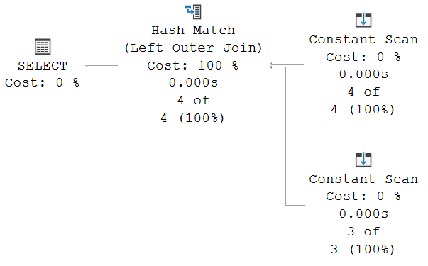
If you really want to make 100% sure that the inputs have not been swapped, then you have to look at the properties of each of the two Constant Scan operators.

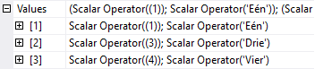
This is what you will see in the Values property of the bottom Constant Scan. This confirms that this is indeed the second input, with the numbers 1, 3, and 4, along with their Dutch names, in the same order as they are listed in the query. Repeating this exercise for the top input shows that the rows with 1, 2, 4, and 6 and their English names are also passed in into the Hash Match operator in the order we typed them in the query.

We can now look at the operation of the Hash Match operator. It first reads its top input, called the build input. On four subsequent calls, it receives the rows for numbers 1, 2, 4, and 6, in that order. These rows are now stored in the hash table, each in the bucket that corresponds to the hash of their Num column, and each stored as unmatched.

Once the entire build input has been processed, the probe phase starts. The first Dutch row is read, which has number 1. Based on the hash of 1, the correct bucket is searched. A match is found. The row for 1 in the hash table will now be marked as having been matched at least once. After that, the operator returns the row to its parent and goes idle.

Once the parent asks for the next row, Hash Match first searches the rest of the bucket to see if there are more matching rows there. That is not the case, so the next row from the probe input is read. This row has number 3. The bucket for whatever the hash of 3 is, is most likely empty. Or, if 3 happens to have a hash collision with one of the values that are in the build input, the bucket is not empty, but none of the rows in it are a match. Either way, the operator does not find matches for this row. And because this is not a right or full outer join, the row is not returned. Hash Match simply discards it, and asks the next row from its bottom input.

This next row is for the value 4. The bucket for the hash of 4 is not empty: the matching row from the English input is there, possibly with other, non-matching rows if there is a hash collision. So now this row in the hash table is also marked as having been matched at least once, and it gets returned.

After that, Hash Match is once more requested to return a row. There are no extra matches for 4 in the rest of the bucket, so Hash Match requests the next row from the probe input. Instead, it receives the end of data signal. At this point, the following rows have already been returned to the client:

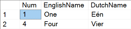
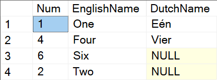
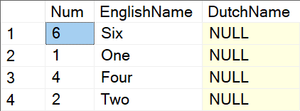
This would of course be the correct result for an Inner Join operation. But we need a Left Outer Join, which means that all unmatched rows from the left input, the English names, need to be returned as well. The Hash Match operator can find these in the hash table. Remember, it started by loading all the English numbers and names in there. While processing and finding matches, the rows with numbers 1 and 4 were marked as matched. The remaining rows, for numbers 2 and 6, have not been matched, and are hence still marked as unmatched. So, to complete the left outer join operation, all Hash Match has to do is run the final phase, where it goes through all the rows in the hash table, skips rows that are marked as matched, and returns those that are marked as unmatched. The final query results then look like this:

Order in the court!

Before I move on, I want to make a very important remark. I am now going to look at the order of the rows. However, I want everyone to remember that, without an ORDER BY at the outermost level of a query, order of results is never guaranteed. And even with an ORDER BY, order of rows that are tied for the order by columns can still be returned in any order.

However, execution plan operators have a very predictable behavior. The lack of order guarantee is because the optimizer might change the execution plan. Or because a new version, or even a cumulative update, changes something. But as long as the execution plan does not change, and nothing externally changes that might influence what happens, behavior is reliable, and we can draw conclusions from the order in which the data is received.

When looking at the result set of this query, or any other query that uses a Hash Match (Left Outer Join) and does not reorder rows returned by it, is confirmation of the process. All matches are found and returned during the probe phase; all retained non-matched rows from the left (or top) input are returned after the probe phase is over, in the final phase. Every Hash Match (Left Outer Join ) always returns all matching rows first, followed by all left-retained rows.

We also see that the first two rows in the output, the matched rows, are in the same order as the probe input, the Dutch numbers. Granted, in this case they are also in the order of the build input. But feel free to play around with the order of the rows in the query. You will find that changing the order of the English numbers and names does not affect the order of the results, whereas swapping rows around in the Dutch input will get reflected in the order of the matched rows in the output. This is not because they get sorted in the execution plan. It is just because the rows happened to be in this order in the input, and none of the operators did anything to change that order.

However, the last two rows, the unmatched and retained rows from the English input, are in what appears to be a random order. Again, feel free to add more rows to the sample query, or change rows, or change their order. Play with it as you wish. You will see that the unmatched rows are always (*) returned in the same order, regardless of input order. And that is because these are returned in the final phase of the Hash Match, where it reads through the entire hash table to find and return any rows that are not yet marked as matched.

(*) Actually, not really always. In the next two parts, I’ll show examples where this is no longer true. But it is very unlikely that you run into these by accident, so I expect you won’t find them by just randomly changing the input data in this query.

I want it all!

So, we now know that, for this query, the value 2 is stored somewhere after the value 6 in the hash table. But we don’t know yet how their positions relate to those of the values 1 and 4, even though they, too, are stored in that hash table. How can we change that?

The answer is simple. The only reason that 1 and 4 were not returned in the final phase is that they were already returned in the probe phase. If I want to know where, relative to the other rows, these are stored in the hash table, all I need to do is to make sure that there are no matches for these rows.

Unfortunately, SQL Server’s optimizer does have some optimizations that, in this case, work against me. If I reduce the probe input to just a single row, then simplification kicks in, and this input gets eliminated. We need at least two rows to make sure that we get an execution plan that actually processes and joins the two inputs. And we also need to make sure that these rows are guaranteed to never be a match for any of the English rows. Using NULL looks like a great way to achieve that – but unfortunately runs into yet another simplification. So what I did instead was to switch to 0. Of course, as soon as you add 0 to the English input, you’ll have to change the Dutch input again. Use any value for the Num column that is not in the English input, and use it twice.

SELECT           English.Num,
                 English.Name AS EnglishName,
                 Dutch.Name   AS DutchName
FROM            (VALUES (1, 'One'),
                        (2, 'Two'),
                        (4, 'Four'),
                        (6, 'Six'))  AS English (Num, Name)
LEFT OUTER JOIN (VALUES (0, 'Nul'),
                        (0, 'Nul')) AS Dutch (Num, Name)
           ON    Dutch.Num = English.Num
OPTION (HASH JOIN, FORCE ORDER);

I won’t show the execution plan here. Apart from the number of rows from the second Constant Scan, it is exactly identical to that of the first query. But now, with the changed second input, we did create the situation we want. Hash Match first, again, stores the rows for numbers 1, 2, 4, and 6 in the hash table. Then it processed the Dutch input, but it won’t find any matches. That leaves all rows in the hash table still marked as unmatched, which means that all four are now returned in the final phase:

And that is our answer. Apparently, the numbers 1 and 4 are stored somewhere in between 6 and 2 in the hash table, with 1 coming before 4.

(Do note that, since the hash functions used by Hash Match are not documented, they are subject to change between versions or even cumulative updates. Or even processor architecture or other properties of your machine. So the results may be different for you.)

Now, is this useful? Nah, not really. Not yet. But we do now have a trick that allows us to see in what order data has been stored in the hash table. The next step is to be very deliberate about what data we put in there, and then use this trick to check the order of that meticulously curated data. That’s what I will do in the next blog on this topic!

One final note

I do want to point out that all of the above hinges on one important assumption: the assumption that, in the final phase, Hash Match reads through the hash table in the most logical order: bucket by bucket, in ascending bucket order. It is, in theory, possible that Microsoft have chosen to read through this in a fully different order.

But that is a rather wild theory. The output from Hash Match is considered unordered, so there is never any reason for the optimizer, or for the engine team who wrote the code for all operators, to prefer a specific order. It makes sense to write the simplest and fastest possible code. And that would be to just start at the first bucket, read it, then move to the next bucket, and so on, until the last bucket has been read. Any other method would complicate and slow down the code, for no benefit. Well, unless Microsoft considers “confusing Hugo” a benefit worth sacrificing performance for.

In case you are still concerned, you will also see, in the next two posts in this series, that all my observations fully confirm that the final phase does indeed go through the hash table one bucket at a time.

Coming next

That wraps up the first part of this series. In the next part, we will use what we learned here to peek into the internal structure of the hash table. After that, we are going to try to use this trick to find hash collisions in our input data.

Once we are done with that, I want to try to find ways to look into the structure of the spilled parts of the hash table, as they are stored in tempdb. To be honest, though I have some ideas on how to approach this, I don’t yet know if they will be successful. So, wish me luck!