Welcome to part eighteen of the plansplaining series. Like the previous posts, this one too focuses on temporal tables and their effect on the execution plan. After looking at data modifications in temporal tables and at querying with a most basic temporal form of temporal query, let’s look at the more advanced variations for temporal querying.

We’re still looking at getting data from a single query only in this post. We’ll look at joins in the next post.

Sample tables

For the code samples in this post, I keep building on the demo tables and sample data from the previous post. If you followed along and have not cleaned up, then you can just keep going. If you need to re-create them, you can use the code below. In that case, do make sure to pause for a bit where the comments indicate it, so that you can (if you wish) stick in the correct timestamps in the sample queries below to get relevant data returned.

CREATE TABLE dbo.Suppliers
    (SupplierID   int          NOT NULL,
     SupplierName varchar(50)  NOT NULL,
     ValidSince   datetime2(7) GENERATED ALWAYS AS ROW START NOT NULL,
     ValidUntil   datetime2(7) GENERATED ALWAYS AS ROW END NOT NULL,
     PERIOD FOR SYSTEM_TIME(ValidSince, ValidUntil),
     CONSTRAINT PK_Suppliers
         PRIMARY KEY (SupplierID))
WITH (SYSTEM_VERSIONING = ON (HISTORY_TABLE = dbo.SuppliersHistory));

CREATE TABLE dbo.Products
    (ProductCode char(10)     NOT NULL,
     ProductName varchar(50)  NOT NULL,
     SupplierID  int          NULL,
     ValidSince  datetime2(7) GENERATED ALWAYS AS ROW START NOT NULL,
     ValidUntil  datetime2(7) GENERATED ALWAYS AS ROW END NOT NULL,
     PERIOD FOR SYSTEM_TIME(ValidSince, ValidUntil),
     CONSTRAINT PK_Products
         PRIMARY KEY (ProductCode),
     CONSTRAINT FK_Products_Suppliers
         FOREIGN KEY (SupplierID)
         REFERENCES dbo.Suppliers (SupplierID),
     INDEX ix_Products_SupplierID NONCLUSTERED (SupplierID))
WITH (SYSTEM_VERSIONING = ON (HISTORY_TABLE = dbo.ProductsHistory));
GO

-- Insert some sample data
INSERT dbo.Suppliers (SupplierID,
                      SupplierName)
VALUES (1, 'Supplier 1'),
       (2, 'Supplier 2'),
       (3, 'Supplier 3'),
       (4, 'Supplier 4'),
       (5, 'Supplier 5'),
       (6, 'Supplier 6');

INSERT dbo.Products (ProductCode,
                     ProductName,
                     SupplierID)
VALUES ('Prod 1', 'Product number 1', 1),
       ('Prod 2', 'Product number 2', 2),
       ('Prod 3', 'Product number 3', 3),
       ('Prod 4', 'Product number 4', 4),
       ('Prod 5', 'Product number 5', 5),
       ('Prod 6', 'Product number 6', 1),
       ('Prod 7', 'Product number 7', 2),
       ('Prod 8', 'Product number 8', 3),
       ('Prod 9', 'Product number 9', 4);
GO

-- Pause here for a minute or so
-- Rename product 4
UPDATE dbo.Products
SET    ProductName = 'New name for ' + ProductName
WHERE  ProductCode = 'Prod 4';
GO

-- Pause here for a minute or so
-- Delete supplier 6
DELETE dbo.Suppliers
WHERE  SupplierName = 'Supplier 6';
GO

Note that the sample data above is severely limited. If you want to make the sample scenarios, queries, and results a bit more interesting, then feel free to simulate some more changes over time. But remember, the focus of this post is not on realistic use cases and credible sample data for temporal tables; I am at this time only interested in how temporal queries work under the cover, to help me better understand their potential performance impact.

Retrieving data with temporal queries

As mentioned in the previous post, the “FOR SYSTEM_TIME” keyword is specifically intended to look at both current and historic data and return not what is valid now, but what is or was valid based on a time specification. The most basic and most commonly used form is FOR SYSTEM_TIME AS OF <date_time>, and we covered that already. Let’s now look at all other variations.

FOR SYSTEM_TIME FROM <start> TO <end>

If you want to see all data that was valid during a specific period (either the entire period or a part of it), then the FROM … TO specification is what you need. It returns all rows that existed for part or all of the specified interval. This includes rows added before the interval and unchanged during the period, as well as rows inserted or deleted during the interval. If a row was changed during the interval, then all versions that were valid during the specified time period are returned. For this reason, queries that use the FROM … TO specification typically include the columns that store the valid period of a row in the SELECT list. Otherwise the output data would contain two or more version of the same row (same primary key value), with no way for the user to know which version was valid at what time.

DECLARE @Start datetime2(7) = '2021-04-03 15:45',
        @End   datetime2(7) = '2021-04-03 15:50';
SELECT p.ProductName,
       p.SupplierID,
       p.ValidSince,
       p.ValidUntil
FROM   dbo.Products
    FOR SYSTEM_TIME FROM @Start TO @End AS p;

I requested an execution plan only for the sample query above. This is what I got:

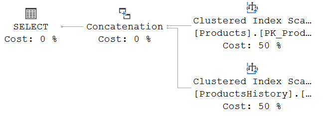
If you compare this to the execution plan that was used for the AS OF query in the previous post, you will see that the same basic pattern is used of reading the current table and the history table separately, then combining the results in a Concatenation operator. In this case, both tables are read with a Clustered Index Scan, which is of course the result of the optimizer looking at the filters used, the available indexes, and the estimated data distribution. Please see my previous post in this series for a longer discussion of the steps taken by the optimizer to come up with an execution plan and the options we have available in the form of indexing to give the optimizer better choices.

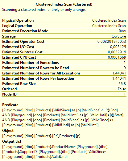
To see the actual difference introduced by using FROM … TO instead of AS OF, we will need to look at the filter used, which can be found in the Predicate property of each of the two Clustered Index Scan operators. (If the optimizer had chosen a Clustered Index Seek, we would have to combined the Predicate and the Seek Predicates).

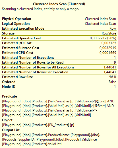Shown to the right are the properties of the Clustered Index Scan operator on, in this case, the current table. (There are no differences between the scans on the current and the history table that are relevant for the discussion here, so I just randomly picked one for the screenshot). The Predicate expression shows how the FROM … TO specification is translated into a filter on the ValidSince and ValidUntil columns in the table. We see three conditions. The first two make perfect sense: “ValidSince < @End AND ValidUntil > @Start” specifies exactly what I described above as “all data that was valid during a specific period”. If the data was removed before the period started, or if it was added after the end of the period, then it was not valid at any time during the period; in all other cases it must have been valid for either a part of or the entire specified period.

But what about that third requirement? Why is “ValidSince <> ValidUntil” added as an extra filter, even though nothing in our query suggests we want this?

Multiple changes in a transaction

To understand why this is required, we actually need to get back to how data modifications on temporal tables are processed. We already looked at the execution plans in this post. For now let’s set the “how” aside and focus on the “what”.

So let’s say we execute the code below:

BEGIN TRANSACTION;
UPDATE dbo.Products
SET    ProductName = 'First change'
WHERE  ProductCode = 'Prod 1';
GO

UPDATE dbo.Products
SET    ProductName = 'Second change'
WHERE  ProductCode = 'Prod 1';
UPDATE dbo.Products
SET    ProductName = 'Final change'
WHERE  ProductCode = 'Prod 1';
COMMIT TRANSACTION;

All of these statements are part of a single transaction. Transactions are all or nothing in relational databases. Intermediate states are assumed to never have happened. So from a logical point of view, looking at committed data only, the name of product ‘Prod 1’ changes from ‘Product number 1’ to ‘Final change’. The values ‘First change’ and ‘Second change’ never exist in a committed state.

The problem SQL Server has is that it does not know which value will be the final value until the transaction is committed. When the first update of the three above executes, SQL Server cannot predict what will happen in the next batch. The second and third updates plus the commit are in a single batch; here at least in theory it might be possible to do some analysis and prediction, but it gets complex fast when conditional statements and various error scenarios come into play.

So instead, each statement just executes individually without knowing whether more changes will follow in the same transaction. The history table still needs to be handled in a way that ensures only the committed changes are seen. The probably most pure way to handle that is to keep all changes in an internal work area and only update the history table when the transaction commits. That introduces a lot of extra logic and requires potentially huge amounts of internal storage, which either eats away internal memory or adds pressure to tempdb. Or we can cheat.

SQL Server cheats.

Step by step

When the first update statement executes, it uses an execution plan similar to the ones we’ve seen before. The end result is that a row is added in the history table with a copy of what was in the current table and ValidUntil set to “now”, then the current table is updated to reflect that ProductName is now ‘First change’, and that this version of the row is valid as of “now”. Except where I write “now”, it doesn’t really use “now” – if you think back of when we looked at the plans for modifications you’ll recall that it uses an internal function “systrandatetime”, which returns the exact time the transaction started (which will in this case probably be just a few milliseconds before “now”).

The second update does effectively the same. So the now current row (with name ‘First change’, and valid since the start of the transaction) is copied to the history table and its ValidUntil is set to the end of the transaction; then the current row is updated to be valid since the start of the transaction (an update that doesn’t actually change anything) and to set the name to ‘Second change’. And then the third update follows the same logic yet again.

So the end result of the transaction is that the values ‘First change’ and ‘Second change’, that logically never existed, do get stored in the history table after all. But because the timestamp is set to the start of the transaction, not the actual clock time of the modification, these versions of the row are stored as being valid for an exact zero duration.

“But Hugo. You said that only committed values should be stored in the history table because these intermediate values never existed at all.”

Ahem. No. I said that only committed changes should be seen when querying history. All of the rules and definitions in the relational model and the SQL standard describe data stored and results returned on a conceptual level. How a vendor wants to build the product, how they want to actually store the data, is left as a vendor choice. If Microsoft wants to store extra data, they can. As long as it’s never returned.

And that’s why the Predicate on the Clustered Index Scan above includes that extra condition: “ValidSince <> ValidUntil”. All rows that represent an intermediate state within a transaction have both ValidSince and ValidUntil set to the start of the transaction. This filter ensures that these rows are not seen. Which exactly meets the requirement that only committed changes should be seen.

Issues

The way SQL Server handles this prevents a lot of complex logic and prevents pressure on either memory or tempdb for transactions that have lots of changes. But it does come with a few issues.

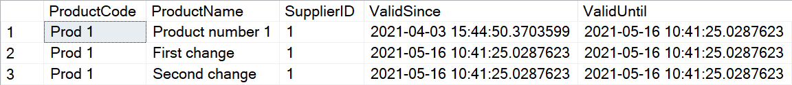
First of all, as mentioned, these intermediate states are assumed to never have existed at all, so they should not be visible ever. But the history table itself can be queried directly. And if you do, you will see these values that never existed, as having existed with zero duration.

BEGIN TRANSACTION;
UPDATE dbo.Products
SET    ProductName = 'First change'
WHERE  ProductCode = 'Prod 1';
GO

UPDATE dbo.Products
SET    ProductName = 'Second change'
WHERE  ProductCode = 'Prod 1';
UPDATE dbo.Products
SET    ProductName = 'Final change'
WHERE  ProductCode = 'Prod 1';
COMMIT TRANSACTION;

Granted, if you look in the documentation on temporal tables you will notice that Microsoft never suggests that the history table can be queried directly. But it is also never explicitly called out as unsupported, and the product does nothing to stop it. I think this is sloppy. The data above should not be visible from querying supported user table.

Second, we know that all intermediate values are guaranteed to have ValidSince equal to ValidUntil. But that doesn’t logically imply that all rows in the history table with ValidSince equal to ValidUntil are guaranteed to be intermediate values. Granted, when the data type used is specified as datetime2(7), the odds are pretty good. But the precision used for these columns is a choice. If I set the precision to datetime2(0), then it becomes painfully easy to execute a bunch of changes, all in separate transactions, within a period of less than a second. Query the table with a FOR SYSTEM_TIME FROM <start> TO <end> qualifier, and many states that have at one time been committed will not be shown. Granted, they are still stored in the history table and can be seen by querying that table directly. But if that kind of query is elevated to a supported scenario, then the intermediate values shown in the screenshot definitely become an error!

It doesn’t stop there. In fact, I saved the best for the last. My final and most serious issue with the way SQL Server handles transactions in the context of history tables is that it falsifies the ValidSince and ValidUntil timestamps. Remember, logically speaking the changes in a transaction are only valid once the transaction commits. Not when it starts. Yet all changes within a transaction are timestamped at the start of the transaction.

Let’s look at a sample scenario. At 10:00, your bank starts a batch process to process a file with payment information it has received. That file is processed as a single transaction. Processing takes 10 minutes. One of the transactions in that file is a debit to my account.

At 10:09, I happen to see an online auction for an item I really want. I’m not sure I can afford it, so I quickly log on to the bank. Perhaps the batch process has not yet updated my account. Or perhaps the bank uses snapshot isolation to prevent blocking. Either way, I see my balance before the payment is processed. It is sufficient, so I confidently make my bid. Two minutes later, the auction ends. The auction site submits my payment to the bank and it is voided because I have insufficient balance. The item is returned to the pool to be auctioned again later.

Another bidder then sues me. They claim I overbid intentionally, in an attempt to cheat them out of the bid. My defence is that it was just bad timing I actually checked my bank balance but another payment was processed after I checked. The plaintiff’s attorney subpoenas records from the bank, which results in a DBA running a temporal query to check my account history.

Remember, the transaction started at 10:00 exactly. SQL Server falsely stores the start of the transaction as the time the old row becomes invalid and a new rows becomes valid, even though all rules in the relational model, and all other behaviour in SQL Server, is based on the idea that a change is only valid after a transaction ends. So the report the bank sends to the court in response to the subpoena falsely states that my balance was reduced at 10:00.

My testimony, under oath, that I checked my balance at 10:09 and the payment was not deducted, is rejected and I get to pay damages to plaintiff. Plus I’m now facing a perjury charge as well.

Thank you very much, Microsoft!

FOR SYSTEM_TIME BETWEEN <start> AND <end>

The syntax for the next way to query history from a temporal table is very similar to that of the previous one. Instead of using FROM and TO, is uses BETWEEN and END.

The functionality is also very similar. In fact, there is only one difference, and it is extremely minor.

When you use a FROM … TO, then neither rows that became invalid at exactly the specified start moment, nor rows that became valid at exactly the specified end moment are included in the result. When you switch to BETWEEN … AND, then the only change is that now rows that became active at exactly the specified end moment will now be included as well. (Rows that lost their validity at exactly the specified start moment are still not included).

DECLARE @Start datetime2(7) = '2021-04-03 15:45',
        @End   datetime2(7) = '2021-04-03 15:50';
SELECT p.ProductName,
       p.SupplierID,
       p.ValidSince,
       p.ValidUntil
FROM   dbo.Products
    FOR SYSTEM_TIME FROM @Start TO @End AS p;

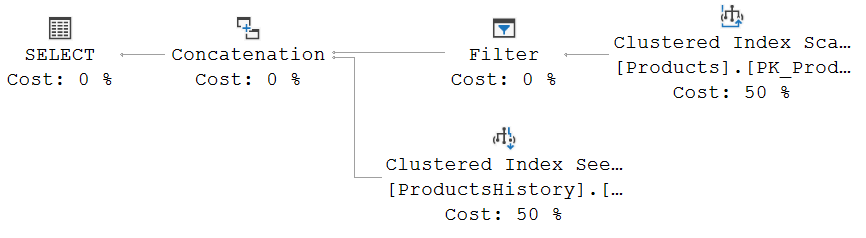
The graphical representation of the execution plan for this sample query looks like this:

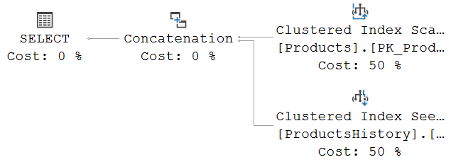
The reason that this execution plan uses a Clustered Index Seek on the history table instead of the Clustered Index Scan we saw in the FROM … TO example is unrelated to the differences between the FROM … TO and the BETWEEN … AND versions of the temporal query specification. The only reason for this change is that I, while investigating multiple changes in a transaction, added three extra rows to the ProductsHistory table. Adding rows to a table affects the estimated costs of scan and seek operators, and that in turn affects plan choice. If you re-run the FROM … TO sample code, you’ll see that this query now also results in a Clustered Index Seek on ProductsHistory.

The only real change between the execution plans for the FROM … TO and the BETWEEN … AND specifications is in the properties. To the right are the properties for the Clustered Index Scan on the current table for the BETWEEN … AND version of the query. And you can be forgiven for not immediately seeing the difference between this screenshot and the previous one. The only difference there is between the two is that one of the three conditions in the Predicate property has changed from “ValidSince < @End” to “ValidSince <= @End”.

And that change matches exactly with the functional changes between the two version. Rows that become valid at exactly the specified end moment are not returned by FROM … TO, but do get returned by BETWEEN … AND.

FOR SYSTEM_TIME CONTAINED IN (<start>, <end>)

Like the previous two, the CONTAINED IN specification also is based on a period. But the functionality here is actually quite different. When using this specification, you request all versions of all rows that have their valid period fully contained in the specified period. This means, rows that became valid on or after the start boundary, and that were invalidated on or before the end boundary.

If a row that already existed before the given period changed once during that period, then it will not be returned. The original version was already valid before the period started, and the updated version was still valid when the period was over. If a row was updated twice during the period, then the version after the first update will be returned: that is the only version that was valid only during the period.

The predicate used to find the correct rows, and it is once more applied to both the current table and the history table, now changes to “ValidSince >= @Start AND ValidUntil <= @End AND ValidSince <> ValidUntil”. Again with the first two conditions to implement the logical condition imposed by the CONTAINED IN specification, and the third condition to ensure that intermediate states that never existed in a committed state are not returned.

But if you look at the execution plan, you suddenly see an interesting change. Let’s use this sample code.

DECLARE @Start datetime2(7) = '2021-04-03 15:40',
        @End   datetime2(7) = '2021-04-03 15:50';
SELECT p.ProductName,
       p.SupplierID,
       p.ValidSince,
       p.ValidUntil
FROM   dbo.Products
    FOR SYSTEM_TIME CONTAINED IN(@Start, @End) AS p;

The execution plan I get looks like this:

Again, the choice between scanning or seeking an index, and which index to use, is entirely based on the normal logic of estimating the number of matching rows versus the total number of rows and using that to cost the operators, as made possible by indexes you may or may not have defined. That’s not what I want to focus on. Instead, I want to focus on the other very visible difference: the Filter operator.

Judging by the graphical representation only, this seems weird. Normally we would expect the Filter to be pushed into the Clustered Index Scan as a residual Predicate property, and then the Filter operator would be removed. Known pushdown blockers such as scalar user-defined functions are not used in this query. So what’s the reason this Filter is not pushed down?

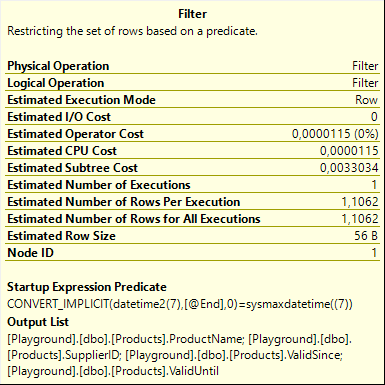The answer is, of course, in the properties. This Filter does not have a Predicate property; instead it has a Startup Expression Predicate property. That means that the operator doesn’t filter individual rows returned to it; it determines during its initialization already whether or not it can return any rows at all. If not, then its child operator never executes.

The condition here reads (simplified) “@End = sysmaxdatetime”. This means that the child operator of this Filter, the Clustered Index Scan on the current table, only executes when the requested period is specified to end at the sysmaxdatetime value, which can be thought of as the logical “end of times”.

And that makes sense, when you think of it. Rows in the current table are always considered to be valid “forever” (or until someone changes the data, whichever comes sooner). If you specify a “real” interval, even when it’s in the future, then any current row can never be contained in that interval because it’s expected to be still valid after the interval ends. Only when you explicitly specify that you are interested in data that is contained in an “interval” that only ends at the end of times, then the current rows might (depending on when they became valid versus the start of the interval) become valid.

If you actually run the query above and request an execution plan plus run-time statistics (what is sometimes erroneously called the “actual” execution plan), then you will see that the Number of Executions property for the Clustered Index Scan remains at zero. The operator never executed. If you add SET STATISTICS IO ON, you will also notice that there are no IOs at all on the current table. Change the value assigned to @End to ‘9999-12-31 23:59:59.9999999’ (the value returned by the ‘sysmaxdatetime((7))’ expression used in the Filter operator), and now the Number of Executions for Clustered Index Scan is 1, and logical reads on this table will be reported by SET STATISTICS IO ON.

FOR SYSTEM_TIME ALL

There is only one temporal modifier left, and this one is pretty simple. FOR SYSTEM_TIME ALL. The name is quite self-explanatory. The keyword ALL means what you expect it to mean: this version will always return the current data and the full history of all rows and all modifications that were ever made (of course, as in all queries, subject to whatever extra filters you might add in the WHERE clause of your query).

Except … well, there is this one little thing. ALL does in the context of temporal table not really mean “all”. Remember those intermediate results that are stored in the history table even though they never exist in a committed state? Remember how they should never be seen?

Exactly. And for that reason, the operators that read data from the current and history tables (most likely scans if there is no additional WHERE clause in the query) still have a single filter left in their Predicate property: “ValidSince <> ValidUntil”.

Conclusion

The FOR SYSTEM_TIME AS OF <date_time> specification we looked at before always returns at most a single version of each row: the version that was valid at the specified moment in time. The specifications we looked at today can all produce zero, one, or more versions of a row, depending on the specification used, the period specified, and when each row started and ceased to be valid.

In all these cases, rows that were valid for a zero duration period are not returned. This is done in order to hide rows that represent an intermediate state of a transaction, and that were not ever valid in a committed state. Logically, the row never was in that state, so it makes sense not to show it. An unfortunately side effect is that very rapid committed changes might also be suppressed because of this logic. This, in addition to the factually incorrect choice to pretend that modifications made in a transaction are valid as of the start of the transaction, rather than the end of it, makes in my opinion the SQL Server implementation of temporal tables far less useful than they might appear at first sight.

For performance tuning, it is important to know how all those temporal tables are translated internally. At one point the optimizer needs to choose which of the available indexes to use, and whether to use seek, scan, or lookup. Those choices depend on the full text of the entire query, including but not limited to the temporal specification. They also depend on the amount of data stored, and the expected selectivity of the various filters (either explicit as a WHERE in the query, or implied by a FOR SYSTEM_TIME specification).

Even though I have now covered all of the aspects of modifying data in and retrieving data from a temporal table, I am still not done with the subject. There will be one more post about temporal tables, where I want to focus on do’s and don’ts of joining data returned from temporal tables.

After that … well, I’ll be honest, I have nothing planned for after that. So, as always, if there is any topic you would like to see covered in a future plansplaining post, just let me know and I will consider it for a future post.