Update February 4, 2026: I have updated this post with new information, about deleted bitmaps, and about the delete buffer for nonclustered columnstore indexes.
Update February 5, 2025: Another update, fairly small in this case. Ordered columnstore indexes were introduced in SQL Server 2022.

In the first part of this series, I described the storage structure and access patterns for SQL Server’s traditional storage structure: on-disk rowstore indexes (heaps and B-trees).

Columnstore indexes were introduced in SQL Server 2012. In that version only nonclustered columnstore indexes were supported (so they stored a copy of the data in the included columns, with the actual table data still stored in an on-disk rowstore heap or clustered index. And they made the table read only! That restriction was lifted in SQL Server 2014, when clustered columnstore indexes were also added. SQL Server 2016 then added the option to create additional nonclustered (on-disk rowstore) indexes on a clustered columnstore. And, also since SQL Server 2016, we now have ordered columnstore indexes – in my opinion a somewhat misleading name.

Note that memory-optimized columnstore indexes, available since SQL Server 2016, will be described in a separate post.

Rowgroups

The data in a columnstore index is subdivided into one or more rowgroups. (If the columnstore index is partitioned, then each partition is subdivided into rowgroups).

When a columnstore index is created or rebuilt, SQL Server will try to fill each filegroup to as close as it can get to its maximum size of 1,048,576 (2 to the power of 20) rows. But there are many circumstances that can cause rowgroups to store less rows than this maximum number.

There are multiple types of rowgroups, that will be described below.

Compressed rowgroup

The performance benefit that columnstore indexes have for analytical queries (many rows but just a few columns from a wide and large fact table) is achieved by the highly optimized storage structure in the compressed rowgroups.

Within each rowgroup of up to 1,048,576, the data is stored in segments. A segment holds the data for a single column of all rows in the rowgroup. So one segment stores all data for the first column, a second segment has the data for the second column, and so on. Each of those segments is compressed, so that far less I/O is required when reading these segments. The actual low-level storage structure used for these segments is in blob pages. That is why the STATISTICS IO output of a columnstore index always includes lob logical reads.

Because each segment stores data from a single column, the likelihood of the same or similar values is high, which greatly increases the efficiency of many compression techniques (such as run-length encoding and dictionaries or variations thereof). SQL Server further enhances this by sorting the rows within a rowgroup for maximum compression efficiency.

However, this sorting can’t be done by column. Since the columns are stored individually, the only way for SQL Server to know which values belong to the same row is by position within the rowgroup. In other words, the SaleDate in position #384,306 of rowgroup 2 is in the same row as the BillDate and the CustomerKey in position #384,306 of rowgroup 2. They are each in their own segment, but must all have the same position. This means that the sorting that is done when (re)building a columnstore index tries to find the best compression over all columns, but can’t optimize each individual column.

For each segment, SQL Server tracks the minimum and maximum value in all of the up to 1,048,576 rows in that segment. This is stored in the metadata of that segment and can be used for rowgroup elimination (described below).

Delta store

Modifying data in a compressed rowgroup would be extremely inefficient. Updating a column would require the affected values to be changed in the appropriate segment. Because of the compression used, this could also affect the stored data for all other data in the segment. For deleting a row, all segments in the rowgroup would be affected, since all columns are deleted. Adding rows is relatively speaking less expensive, but still rather expensive: while the new values could be added at the end of a compressed rowgroup that still has room, there is still a lot of work involved in ensuring that the new data gets correctly compressed, since many compression methods are based on previous values.

That high cost of modifying compressed rowgroups is why tables with columnstore indexes were read-only in SQL Server 2012. To modify the table, we had to drop the columnstore index, run the modification, then recreate the index again. Which was of course very cumbersome. That is why Microsoft lifted the read-only limitation in SQL Server 2014. However, the modifying compressed rowgroups is still prohibitively expensive. For that reason, Microsoft “cheated”. The compressed rowgroups are still read-only, and modifications are tracked in a different way.

When rows are inserted, they are added to a so-called open rowgroup. This means that they are stored in a regular on-disk rowstore clustered index. The key for the clustered index is not any column from the data, but a row number that is internally generated. Just like compressed rowgroups, open rowgroups are also limited to 1,048,576 rows. Once that number is reached, the rowgroup is marked as closed, and a new open rowgroup is created for more inserts.

An asynchronous process, called the tuple mover, looks for closed rowgroups, and compresses them. That replaces the closed rowgroup with a compressed rowgroup.

Note that the above process only applies for so-called “trickle insert”. For any bulk load where 102,400 rows or more are added through the Bulk Insert API, they will be put in a new rowgroup and instantly compressed. Smaller batch sizes, even through the Bulk Insert API, are still added to an open rowgroup.

When you delete a row that is in a compressed rowgroup, it is not actually deleted from the compressed segments. Instead, they are tracked in the deleted bitmap. This name is somewhat misleading: while it is indeed stored as a bitmap in memory, it is persisted on disk as a B-tree index on a compound column: the position of each deleted row in the rowgroup. So if we would run a delete for the row that is stored in position #384,306 of rowgroup 2, the value (2; 384,306) will be stored in the B-tree of the deleted bitmap. The data for the row is still in the compressed rowgroup (so that we don’t have to modify the data here), but marked as deleted, which means that execution plan operators will not process this row.

Note that the minimum and maximum values of the affected segments, as stored in the metadata, are not affected. Even if the deleted row happened to have the minimum or maximum value, SQL Server will not rescan the entire segment to find the new minimum or maximum value.

When rows in a compressed rowgroup are updated, SQL Server simply combines the methods for deleting and inserting data. The existing row is marked as deleted in the deleted bitmap, and a new row with the now current values is added to an open rowgroup. There is no bulk update process that would instantly compress the rowgroup, so even when an update affects millions of rows, they are all added through the trickle insert process, and then asynchronously compressed by the tuple mover.

When a lot of data has changed, it can be useful to rebuild the columnstore index. This will actually remove the data for all the deleted and updated rows, resort each rowgroup for optimal compression, and find the new correct minimum and maximum value in each segment.

All of the above (open and closed rowgroups, plus the deleted bitmap) is collectively called the delta store. Every columnstore index has a delta store, and a partitioned columnstore index even has a separate delta store for each partition.

Clustered or nonclustered

Most of the above description applies equally to both clustered and nonclustered columnstore indexes. However, there are some important differences.

The first difference is, of course, the data included. A clustered columnstore index, like any clustered index, is the table, so it always stores all columns in the table. For a nonclustered columnstore index, you specify which columns to include in the index, and then the index holds a copy of the data, for the specified columns only. With one exception. Whether specified or not, a nonclustered columnstore index will always include all columns that are needed to locate the row in the table. If the table has a clustered index, that means all columns of the clustered index, including the uniqueifier (if any). If the table is a heap, the RID (see my previous post) will be in the nonclustered columnstore index, as a hidden column.

The other big difference between clustered and nonclustered columnstore indexes is how deleted data (and remember, that includes the old version of updated rows) is handled. For nonclustered columnstore indexes only, this involves one additional structure in the delta store: the delete buffer. Like the deleted bitmap, this is also a list of rows that were deleted but have not yet been removed from the compressed rowgroup. However, where the deleted bitmap tracks the deleted rows by their ColStoreLoc (rowgroup number and position within that rowgroup), the delete buffer stores a logical identification for those deleted rows: the clustered index key or RID.

So why this extra complexity? The reason is: performance. And especially the performance of delete statements.

Many delete statements on a table with a nonclustered columnstore index will be based on a filter in a WHERE clause. Which means that, hopefully, the rows to be deleted will be found by seeking one of the rowstore indexes, not by scanning the complete nonclustered index. Each and every one of those rowstore indexes includes the column(s) to identify the row: the clustered index key, with uniqueifier if needed, or the RID. But they do not include the location of the row in the nonclustered columnstore. That would be impractical, because that location might change when the index is rebuilt, or even when an open rowgroup is closed and then compressed. We don’t want such changes to require all rowstore indexes to be modified as well. So, except for the rare cases where the rows to be deleted are found in a Columnstore Index Scan, the engine has no clue where the affected rows are in the index. Which means we can’t add their location to the deleted bitmap.

If we want to get that location, we’d have to do a full scan of the nonclustered columnstore index. For each deleted row. That is absolutely not efficient. And that is why the delete buffer exists. We do have the clustered index key or RID, because those are included in every rowstore index. So we can store that clustered index key or RID in the delete buffer.

As the number of deleted rows grows, this becomes less efficient. That’s why the tuple mover, the background process that compresses closed rowgroups, also looks at the size of the delete buffer. If there are over 1,048,576 rows in there, it will compare the compressed rowgroups to the delete buffer, joining them on the clustered index key or RID, to find the location of each row in the delete buffer, mark that row as deleted in the deleted bitmap, and then remove it from the delete buffer.

Ordered columnstore

A common best practice is to force the data to be in a specific order before building (or rebuilding) a columnstore index, for instance by first creating a rowstore clustered index. This does not cause the data within each rowgroup to maintain that order (remember, each rowgroup is ordered to achieve optimal compression). But it does affect what rows go into which rowgroup, which, when well designed, can improve the efficiency of rowgroup elimination (see below).

To make this process easier, Microsoft introduced ordered columnstore indexes in SQL Server 2022 (for clustered columnstore indexes) and SQL Server 2025 (for nonclustered columnstore indexes). Despite what the name suggests, the data in these indexes is still unordered. The only thing that is different for an ordered columnstore index in comparison to a regular one, is that SQL Server will automatically order the data before building (or rebuilding) the compressed rowgroups, to get optimal minimum and maximum values in each segment, for more efficient rowgroup elimination. Within each rowgroup, the data is then still reordered to optimize compression. And future modifications are still handled exactly as for regular columnstore indexes. Only a rebuild will then, once more, cause the data to be sorted before building the new compressed rowgroups.

Reading from a columnstore

Now that we know how the data in a columnstore index is structured, let’s look at how the data can be read into an execution plan.

Columnstore Index Scan

When you see a Columnstore Index Scan in an execution plan, the frontend tool you use is actually lying to you. It is just an Index Scan in the execution plan XML, but with the Storage property set to Columnstore. Several frontend tools recognize this Stoareg property, to then display a different icon and operator name.

A Columnstore Index Scan minimizes the work it needs to do in two ways:

• Column elimination: based on the Output List and Predicate properties, it only accesses segments that store data for columns that need to be returned, or that are used in a filter that is pushed into the scan. The segments for all other columns are not used at all. Column elimination only applies to compressed rowgroups, since open and closed rowgroups are stored row by row in a B-tree.
• Rowgroup elimination (often mistakenly called segment elimination): for each condition in the Predicate property, SQL Server looks at the minimum and maximum value in the metadata of each compressed rowgroup. If this is such that none of the rows in the rowgroup can qualify, then the entire rowgroup is skipped. Rowgroup elimination only applies to compressed rowgroups, since the minimum and maximum value are not stored in the metadata for open and closed rowgroups.

For the remaining rowgroups, all relevant segments plus the deleted bitmap are read in sync, and each combination of values from these is returned, unless the deleted bitmap marks the row as deleted, or unless the Predicate property causes the row to be rejected. Of course, open and closed rowgroups are also scanned and returned. This uses the same process as for an Index Scan on a regular on-disk rowstore index. Finally, the data is returned in batches, rather than row by row, when the Columnstore Index Scan is running in batch mode.

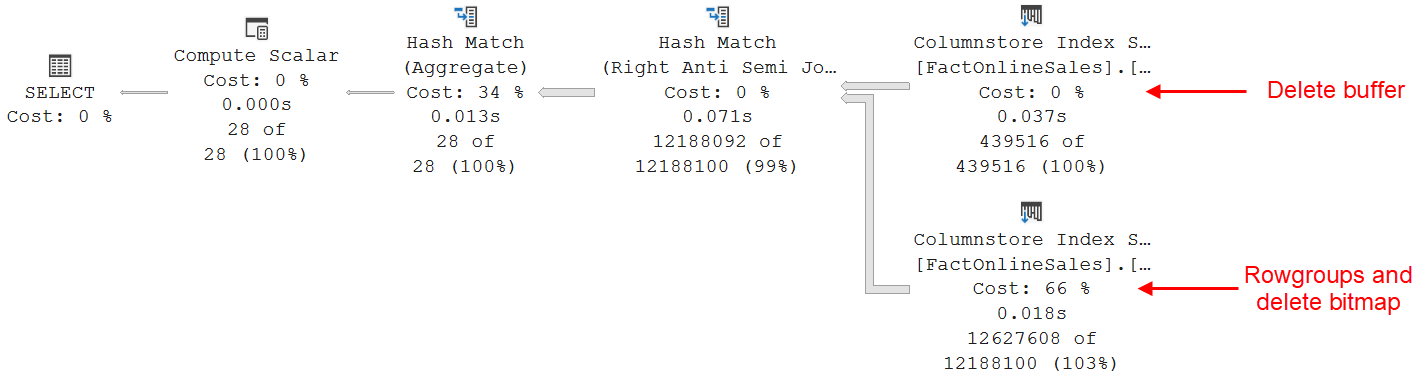
For nonclustered columnstore indexes that have a non-empty delete buffer, this process is insufficient. We still need to filter out the rows that are marked as deleted in that delete buffer. This is not done in the Columnstore Index Scan itself. So, all the rows that are marked as deleted in the delete buffer (as opposed to the deleted bitmap) are returned. They are then joined to a separate scan of the delete buffer. That join uses an Anti Semi Join operation, which causes rows from the columnstore that also exist in the delete buffer to be removed from the final result. All this extra work is not visible in the execution plan. Microsoft decided to hide this from us. However, if you enable trace flag 8666 (which is very definitely NOT recommended for production usage, unless instructed by Microsoft support staff), you can actually see the real execution plan.

Please note that a Columnstore Index Scan does not properly report it’s logical reads in its Actual I/O Statistics property. The values here are always reported as zero. To see the amount of work done by a Columnstore Index Scan, you need to use SET STATISTICS IO ON. And in the output, make sure to not only look at logical read, but also at lob logical reads.

Because the data in a columnstore index is not ordered (even for an ordered columnstore index), the Ordered property of a Columnstore Index Scan is always False.

No Columnstore Index Seek

Columnstore indexes are not designed for fast retrieval of specific rows. As a result, SQL Server does not support seek operators on columnstore indexes.

Key Lookup

A Key Lookup is effectively the same as a Clustered Index Seek. As such, one might expect that a Key Lookup is not supported on a columnstore index either. And until SQL Server 2014, that was true. However, that was changed in SQL Server 2016.

A nonclustered index on a table with a clustered columnstore index will, in its leaf pages, store the location within the columnstore index of each row. This is called the ColStoreLoc in execution plans. While undocumented, I assume this to be a combination of rowgroup number and ordinal position within the rowgroup.

A Key Lookup on a columnstore index will first perform the same column elimination and rowgroup elimination as a Columnstore Index Scan. However, since a Key Lookup is always called for a single ColStoreLoc, it only tries to eliminate the specific rowgroup mentioned, and when successful, will read nothing at all.

If the rowgroup can’t be eliminated, Key Lookup will read the necessary rowgroups and decompress them. Because of how compression works, this involves at least decompressing all rows before the required row. So if we happen to search for row 20 in a rowgroup, this is not a huge problem. For row 964,491, though, it is an enormous task! As a result, the optimizer will only choose for a Key Lookup strategy if the supporting nonclustered index provides an extremely selective filter.

Just as for the Columnstore Index Scan, a Key Lookup on a columnstore index doesn’t give any information in the Actual I/O Statistics property; you need to look at logical reads andlob logical reads in the SET STATISTICS IO ON output.

Conclusion

SQL Server supports up to one columnstore index on a table. While the clustered version is usually preferred, nonclustered is supported as well.

The data in a columnstore index is compressed and optimized for fast retrieval of a subset of the columns for large number of rows – no filter, or a not very selective filter. This is then done by the Columnstore Index Scan, that scans through each rowgroup that can’t be eliminated.

While a Key Lookup on a clustered columnstore index is supported, it is a very inefficient way to access the data, and it will only be chosen by the optimizer if it estimates the filter on the nonclustered index to be extremely selective.

That concludes this very high level and broad overview of columnstore indexes. In the next episode, I will cover memory-optimized indexes.