This is part twenty-four of the plansplaining series. In the previous part, I explained the execution plans for basic window functions, with and without a window frame. Especially the latter group performed quite poorly in the examples. So let’s now look at an optimization that SQL Server can apply to most cases, that prevents this rather bad scaling.

Running totals

The examples in the previous post all used a window frame that started at (some number) PRECEDING. And as long as (some number) is quite low (and the end of the frame is not defined as (huge number) FOLLOWING), the performance impact that is caused by the Window Spool operator replaying the entire frame for each row remains within acceptable limits. It only starts to hurt when the window frames get really large, like in the examples I used, with values such as 9999 PRECEDING or 10000 PRECEDING.

But real use cases of framed window aggregations that need such large frames are, in my experience, extremely rare – with one very important exception. And that exception is when the start of the frame is specified as UNBOUNDED PRECEDING. This means that the frame starts at the first row of the partition, and keeps growing, no matter how many more rows there are. This is in fact very common, perhaps the most used use case for framed windows, especially in the form BETWEEN UNBOUDED PRECEDING AND CURRENT ROW, the window frame specification that computes running total, running tally, running average, etc.

The frame for running aggregation is theoretically unlimited. A partition could have a million rows, and in that case the frame for the last row would contain all those million rows. And based on the description in my previous post, you would probably expect Window Spool to store those million rows, and to return all to its parent Stream Aggregate, so that it can compute the result of the aggregate function.

Luckily, this is not the case. Let’s modify one of the examples from the previous post a bit. The only change is that the starting point is now UNBOUNDED PRECEDING, instead of 10000 PRECEDING as in the previous post:

SELECT   p.ProductID,
         p.Name,
         p.ListPrice,
         p.ProductLine,
         MAX (p.ListPrice) OVER (PARTITION BY p.ProductLine
                                 ORDER BY p.ListPrice
                                 ROWS BETWEEN UNBOUNDED PRECEDING
                                          AND CURRENT ROW) AS RunningMax
FROM     Production.Product AS p;

If you execute this query with the SET STATISTICS TIME and SET STATISTICS IO options enabled, you will notice that this version runs a lot faster. And you will notice that there are now no logical reads on the worktable.

Table 'Worktable'. Scan count 0, logical reads 0, physical reads 0, [...]
Table 'Product'. Scan count 1, logical reads 15, physical reads 0, [...]

 SQL Server Execution Times:
   CPU time = 0 ms,  elapsed time = 51 ms.

Completion time: 2023-11-18T13:42:43.2084654+01:00

The execution plan with runtime statistics for this query looks, at first sight, identical to the execution plan for the almost-identical query in the previous post:

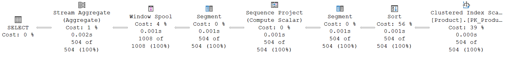
(Click on the picture to enlarge)

But if you look closer, paying attention to the details, you will see one very important difference. The number of rows that Window Spool returns to Stream Aggregate has decreased, from 37,399 when the window frame started at 10000 PRECEDING, to just 1,008 now that the frame is essentially limitless.

(Another difference you may notice is that the Compute Scalar operator that computed TopRowNumber1003 in the previous post is missing here. With UNBOUNDED PRECEDING, the top row number is always 1, and there is no need to compute it and pass it from operator to operator. The absence of a top row number column in the input to Window Spool tells this operator to start each frame at the first row of the partition.)

Fast-track optimization

The Actual Number of Rows that Window Spool returns in the execution plan above is quite a surprise. When the window frame was limited to 10,000 rows, the operator had to return over 37,000 rows. That collection of rows consisted of 504 groups, one for each row from its input. Within each group, the first row was the current row, followed by all rows that were visible in its input frame.

Now that we have removed the boundary on the 10,000^th preceding row, we would expect that each frame is either just as large or has even more rows. So we would expect the number of rows returned by Window Spool to go even further up. The reason that it doesn’t, is because of an optimization that Microsoft implemented specifically for the common use case of “running” aggregations (all aggregations that are specified with ROWS BETWEEN UNBOUNDED PRECEDING AND something): fast-track optimization.

The basis of fast-track optimization is that, for each row, the window frame to use is the same as the window frame for the previous row, plus one extra row. This ties nicely with the internals of how Stream Aggregate works: it has internal counters for the aggregation of all rows processed so far, that it updates for each new row, so that they are the correct aggregate when all rows have been processed. In the context of a running aggregate, this can be very neatly “abused”. The standard computation of the running aggregate for row n is to process rows 1 through n. Or put differently, to process rows 1 through n – 1 (which is the running aggregate for row n – 1), and then process row n. But since we just computed the running aggregate for row n – 1, we don’t need to repeat that. If we don’t reset the internal counters after returning the running aggregate for row n – 1, then we merely need to process one extra row, row n, to get the running aggregate for that row.

This observation is used in the execution plan by modifying the behavior of two operators: Window Spool and Stream Aggregate.

When fast-track optimization applies, Window Spool still returns a group of rows for each input row. However, this group of rows now does not consist of the current row and then all rows in the entire window frame, but only of the current row and then the row (or rows) that have to be added to the previous window frame within the same partition (segment). That is why the Actual Number of Rows in the execution plan above is 1,008, exactly twice the number of rows in the input. Because each group consists of the current row, and then the row that is added to the frame (in this case also the current row).

Stream Aggregate also changes its behavior when fast-track optimization applies. When the partition changes (indicated by column Segment1004, which was produced by the Segment operator to signal the start of a new partition), it initializes all its internal counters as normal. But when the partition does not change, then a change of the Group By column (WindowCount1005) does not initialize all internal counters. Only the internal counters for the ANY function are initialized in this case, which sets them to the values of the first row in the group, which is the “current” row. All other internal counters are left unchanged, so they are still at the running value for all rows of the last row’s frame. After ignoring the first (“current”) row and processing the next row or rows in the group, they are then at the running value for the current row, which is the intended value.

Limited visibility in the execution plan

Unfortunately, there is no easy way to see in the execution plan when fast-track optimization is used. I assume that in the actual, internal implementation of the execution plan, there are properties on both the Stream Aggregate and the Window Spool operator to tell them to change to the modified behavior for fast-track optimization. However, those properties are not exposed in the execution plan XML that SQL Server returns when an execution plan is requested, nor in the graphical representation of that execution plan in the client tools.

However, it is also, at least theoretically, possible that Window Spool does not use an explicit property to decide when to use fast-track optimization, but bases this purely on the presence or absence of a top row number in its input. If this column is not in the input, then the default top row number is used, 1, which means UNBOUNDED PRECEDING, and fast-track optimization can be used. However, from an engineering point of view, I myself would definitely not like a design where such a decision hinges on recognizing a specific column from its name. Plus, the top and bottom row numbers are not passed to Stream Aggregate anyway, so this operator would then still need an explicit property to control whether or not to switch to its modified fast-track mode.

Different end points

The most common use case for fast-track optimization is of course the “classic” running total: aggregation OVER (ROWS BETWEEN UNBOUDED PRECEDING AND CURRENT ROW). But the same optimization technique can also be used when the end of the frame uses the value PRECEDING or value FOLLOWING specification.

Such as for example in this query:

SELECT   p.ProductID,
         p.Name,
         p.ListPrice,
         p.ProductLine,
         MAX (p.ListPrice) OVER (PARTITION BY p.ProductLine
                                 ORDER BY p.ListPrice
                                 ROWS BETWEEN UNBOUNDED PRECEDING
                                          AND 3 FOLLOWING) AS RunningMax
FROM     Production.Product AS p;

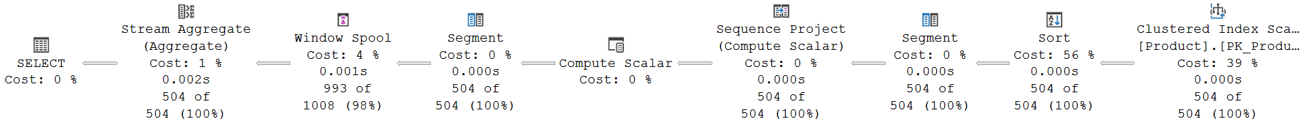
This is the execution plan:

(Click on the picture to enlarge)

The Compute Scalar is back in this execution plan. Not to compute a top row number, but to compute the bottom row number: BottomRowNumber1003 = RowNumber1002 + 3. That makes sense of course. Window Spool defaults to using the current row as the bottom row of the window frame, so it needs to be supplied a bottom row number if the frame ends at another row.

The Actual Number of Rows returned by Window Spool is still only 1,008, because fast-track optimization is still used. In this case, the first row within each partition results in a group of rows that consists of that first row (the current row), followed by rows one through four (the window frame). For the second row, the group then consists of that second row as the current row, and then only the fifth row, which is the row that gets added to the frame. The last few rows of each partition then only return the current row and nothing else as their frame, because there are no more rows within the partition that can still be added to the frame.

For a running aggregate that stops before the current row, the same basic process is applied:

SELECT   p.ProductID,
         p.Name,
         p.ListPrice,
         p.ProductLine,
         MAX (p.ListPrice) OVER (PARTITION BY p.ProductLine
                                 ORDER BY p.ListPrice
                                 ROWS BETWEEN UNBOUNDED PRECEDING
                                          AND 3 PRECEDING) AS RunningMax
FROM     Production.Product AS p;

(Click on the picture to enlarge)

This time the Actual Number of Rows returned by Window Spool is slightly less. That is because the first three groups of rows returned within each partition are just the current row, and nothing else yet: the window frame these rows see is still empty. The fourth row is the first one that adds a row (the first one) to the frame. Every other row in a partition then adds one more. The last three rows of each partition are not visible in any frame, and hence only returned as “current” row by Window Spool, but never as “row to be added to the current frame”.

Both of the previous examples require Window Spool to store some rows in its worktable: either the rows between the current row and the end of the frame (for FOLLOWING), or the rows between the end of the frame and the current row (for PRECEDING). In the former case, the operator also effectively reads ahead a few rows. Just as with “normal” Window Spool processing (no fast-track processing), this worktable is stored in memory when it is guaranteed to never exceed 9,999 rows, or in disk otherwise. So the cutoff point here is at 10000 PRECEDING or at 10000 FOLLOWING.

Fast-track for moving aggregates

We have seen above how fast-track optimization is used for running aggregates, both the standard type (ending at the current row), or the modified versions that end a few (or a lot of) rows before or after the current row. In the previous post, we looked at moving, rather than running, aggregations. And no fast-track optimization was used there. However, depending on the circumstances, there are cases where SQL Server can still use fast-track optimization, even though a query requests moving aggregations.

How, you may ask? After all, fast-track optimization works is only possible by exploiting the fact that running aggregations only add to the frame, and that is exactly what is not the case in moving aggregates.

Let’s find out. I’ll once more modify one of the queries from the previous part a bit. This time, I change it from a moving maximum to a moving average. The rest is unchanged.

SELECT   p.ProductID,
         p.Name,
         p.ListPrice,
         p.ProductLine,
         AVG (p.ListPrice) OVER (PARTITION BY p.ProductLine
                                 ORDER BY p.ListPrice
                                 ROWS BETWEEN 10000 PRECEDING
                                          AND CURRENT ROW) AS MovingAverage
FROM     Production.Product AS p;

The execution plan is still a long line of operators. In fact, it is a much longer line of operators than any of the previous examples! So long that, for readability, I have split it across two lines. So in the picture below, beware that Segment #7 is actually to the right of Sequence Project #6.

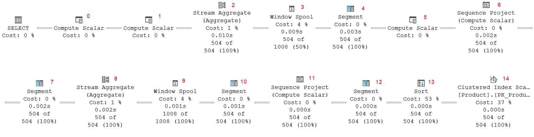
(Click on the picture to enlarge)

What happens here in this execution plan is far from trivial, so let’s approach it systematically, one step at a time. We’ll follow the data, so we will start at the far right.

Reading and sorting the data

The two right-most operators are no surprise. We have seen them in every execution plan for the examples in this post, and for most in the previous post. Clustered Index Scan #14 is used to read all data from the Product table. A scan makes sense in this case, because the query has no WHERE clause to filter on a subset of the rows only. And since there is no nonclustered index that covers this query, scanning the clustered index is the best option. But the data is returned in an order that is useless for computing the window functions, so then the Sort operator (#13) returns the data in order of ProductLine (the PARTITION BY column) and ListPrice (the ORDER BY column).

First window frame aggregate

Operators 12 through 8 form a familiar pattern. We have seen this same pattern in all previous examples. Some of them had a Compute Scalar operator as well, others (like this pattern here) did not. So it looks as if this part of the execution plan computes aggregation for a framed window.

But assumption is the mother of all mistakes, so let’s not assume, but actually check. That should also help us understand exactly what aggregation is computed, and over exactly what window and frame specification.

I’ll run through this quickly because it is essentially a repeat of what we saw in the previous post. I will only go into a bit deeper detail when there are interesting differences.

So, at the right, Segment #12 marks a change in the Group By column, ProductLine; and Sequence Project #11 then computes RowNumber1010 as the row number of each row within every segment (partition). No surprise here.

Segment #10 once more (redundantly, but we have seen that before) computes a segment column to mark changes in ProductLine. Then we get the by now familiar Window Spool and Stream Aggregate pair, #9 and #8. The input has neither a top row number column, nor a bottom row number column. So the defaults apply: the top row number is 1 and the bottom row number is the current row number. This effectively defines the window frame as ROWS BETWEEN UNBOUNDED PRECEDING AND CURRENT ROW. For this definition, fast-track optimization can be used, so it is no surprise to see that this Window Spool returns 1,008 rows, 2 for each of the 504 input rows.

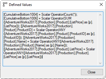The Defined Values in Stream Aggregate #8 then shows that it returns a bunch of columns from the “current” row of each window frame, using the ANY aggregate function. But it also computes two new columns that are actual aggregations. CumulativeBottom1004 is computed using the Count(*) function, and CumulativeBottom1005 is defined as SUM(ListPrice).

The computation of a SUM and a COUNT are not surprising. We already know that SQL Server always computes an average by first computing the sum and the count, and then dividing these to get the average. But what is surprising, is that these are computed as the running sum and running count, from the start of the partition up to the current row. The query does not ask for these values. So why are these computed? And why are the columns for the result named with “CumulativeBottom” as the mnemonic name, rather than the generic Expr that is usually used?

Let’s put those questions aside for now. Hopefully, things will make more sense once we have looked at the rest of the operators.

Second window frame aggregate

Segment #7 and Sequence Project #6 once more compute a row number, while respecting partition (segment) boundaries on a change of ProductModel. The result, RowNumber1008, is always exactly the same as RowNumber1010 that was already computed by Sequence Project #11, so this is a missed opportunity for the optimizer to make this query a tiny bit faster.

The next operator, Compute Scalar #5, then computes BottomRowNumber1009 as RowNumber1008 – 10001. To the left of that, in operators #4, #3, and #2, we once more see the familiar pattern of a (redundant) Segment operator, a Window Spool operator, and a Stream Aggregate operator. There once more is no top row number in the input to Window Spool, so it defaults to 1. The bottom row number is specified in this case. So this time, the Window Spool is used to create window frames defined as ROWS BETWEEN UNBOUDED PRECEDING AND 10001 PRECEDING. Based on that window frame, Stream Aggregate then computes yet two extra columns: CumulativeTop1005 = Count(*) and CumulativeTop1007 = SUM(ListPrice). All other columns are once more taken from the “current” row, by using ANY.

So at this point, we have two different columns that each store a COUNT(*), and two different columns that each store a SUM(ListPrice), but neither is computed using the window frame as specified in the query.

Final computation

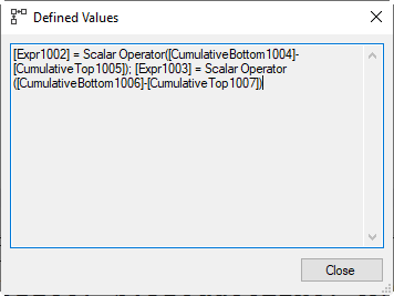All the pieces come together in the last two operators. And the most important part of the puzzle is in Compute Scalar #1. It computes two expressions. Expr1002 is computed as CumulativeBottom1004 – CumulativeTop1005, and Expr1003 as CumulativeBottom1006 – CumulativeTop1007. Let’s look at the last in a bit more detail.

Now, we already know that CumulativeBottom1006 is computed, in Stream Aggregate #8, as SUM(ListPrice) OVER (ROWS BETWEEN UNBOUNDED PRECEDING AND CURRENT ROW). And we also know that CumulativeTop1007 is computed, by Stream Aggregate #2, as SUM(ListPrice) OVER (ROWS BETWEEN UNBOUNDED PRECEDING AND 10001 PRECEDING). So, what is the effect of subtracting these? Let’s say that the current row is row number 15,000 within its partition. CumulativeBottom1006 holds the sum of all ListPrice values in rows 1 through 15,000. CumulativeTop1007 is the sum of all ListPrices for rows 1 through 4,999. Subtract these, and the result is the sum of all ListPrice values in rows 5,000 through 15,000 – and that is exactly the window frame that the query requests! Expr1002 then uses the same method to compute the COUNT(*) for that same window frame.

(I don’t know why, but in my head this becomes more intuitive with smaller numbers. I can easily grasp that the sum of the fifth through tenth value in a range can be computed by finding the sum of the first ten elements, and then subtracting the sum of the first four. And while this seems less effective when explained like this, it can actually be more effective if you happen to have a very efficient way to compute the sum of the first n values – such as fast-track optimization).

Compute Scalar #0 is no surprise anymore at this point. It simply divides the SUM (in Expr1003) by the COUNT (in Expr1002) to find the AVG, with some additional logic to prevent run-time errors when Expr1002 is 0. That is impossible in this case, but it is included in the standard pattern for AVG evaluation, and there is no measurable benefit in removing it in cases where the COUNT cannot be zero.

Summary

Putting this all together, the optimizer has effectively used two transformations to get from the query as specified in the execution plan. The first is the standard transformation of AVG(ListPrice) to SUM(ListPrice)/COUNT(ListPrice). The second is a trick that replaces a single framed window aggregation that does not qualify for fast-track optimization with a set of two different framed window aggregations that both do qualify.

Limitations

The transformation of a single non-fast-track framed window into a subtraction of two different fast-track framed windows is not always possible. There are two conditions that must be met. One is a purely functional restriction. The other is a performance choice.

The first condition relates to the specific aggregate function used. The logic described above that makes this trick work does not apply for all aggregate functions. It works fine for functions such as SUM, COUNT, or Count(*), which is why the example above worked. But it does not work for aggregate functions such as MAX, MIN, or STRING_AGG. You can not find the maximum value in items #5 through #10 by subtracting the maximum found in the first four from the maximum found in the first 10.

There is no official documentation on this that I know of, but as far as I know, this trick only works for SUM, COUNT, or Count(*). For all other aggregate functions, this trick does not work.

However, do note that many T-SQL aggregate functions are computed from SUM and COUNT (such as AVG, that we already saw, but also STDEV, STDEVP, VAR, and VARP), so those aggregates in a query can still result in an execution plan that uses this trick to transform a single moving aggregate to the difference of two running aggregates for which fast-track optimization applies.

The second condition is performance related. The price of replaying the window frame for each current row correlates with the (maximum) size of that window. If that size is sufficiently small, then the overhead of computing two instead of just one running aggregate may exceed the cost saved by not having to compute the moving aggregate the “standard” way. For this reason, the optimizer uses a cut-off point of four rows for this transformation. So if the maximum window frame size is four or less rows (e.g. ROWS BETWEEN 1 PRECEDING AND 2 FOLLOWING), then this transformation will not be applied. If the window can contain five or more rows (e.g. ROWS BETWEEN 1 PRECEDING AND 3 FOLLOWING), then the transformation will be used, if the aggregate functions that are required qualify.

Conclusion

In this post, we saw how fast-track optimization slightly modifies the operation of both the Stream Aggregate and the Window Spool operator, to implement a much more efficient method to compute running aggregates for a framed window aggregate. We then also saw the transformation that the optimizer can use, when the right conditions are met, to replace a single, expensive framed window aggregate for moving aggregates with two cheaper, fast-track optimized window aggregates for running aggregates.

I am not done yet with the OVER clause. There is way more to tell about the execution plans that are generated when you use this clause in a query. But that is for a future episode.

As always, please do let me know if there is any execution plan related topic you want to see explained in a future plansplaining post and I’ll add it to my to-do list!