This is part twenty-six of the plansplaining series. And already the fourth episode about window functions. The first of those posts covered basic window functions; the second post focused on fast-track optimization for running aggregates, and the third post explained how the optimizer works around the lack of execution plan support for UNBOUNDED FOLLOWING.

But all of those were about OVER specifications that use the ROWS keyword. Let’s now look at the alternative, the RANGE keyword.

RANGE instead of ROWS

When a RANGE specification is used, then number PRECEDING and number FOLLOWING are not allowed. So this leaves us with only a few possible RANGE specifications. And even of that limited list, not all need to be discussed.

For instance RANGE BETWEEN UNBOUDED PRECEDING AND UNBOUNDED FOLLOWING means, just as ROWS BETWEEN UNBOUDED PRECEDING AND UNBOUNDED FOLLOWING, that the entire window is visible. There is no frame, and the optimizer will simply pretend you never specified one.

Also, RANGE BETWEEN CURRENT ROW AND UNBOUNDED FOLLOWING is handled the same way as any ROWS BETWEEN CURRENT ROW AND UNBOUNDED FOLLOWING: the optimizer reverses the specified sort order, and then also has to reverse the window frame to RANGE BETWEEN UNBOUNDED PRECEDING AND CURRENT ROW.

RANGE BETWEEN UNBOUNDED PRECEDING AND CURRENT ROW

Using RANGE instead of ROWS for the window frame specification means that a CURRENT ROW endpoint does not necessarily end at the current row. If there are duplicates in the ORDER BY column (or columns), then the end point of the window frame is the last row with the same values in the ORDER BY column(s) as the current row. So for ORDER BY values are unique, RANGE or ROWS do the same. But when there are duplicates, then a RANGE specification includes a few extra rows. You can see the effect of this by uncommenting the RunningSum column in the code below, and then comparing the data in the two columns.

SELECT p.ProductID,
       p.Name,
       p.ListPrice,
       p.ProductLine,
       --SUM (p.ListPrice) OVER (PARTITION BY p.ProductLine
       --                        ORDER BY p.ListPrice
       --                        ROWS BETWEEN UNBOUNDED PRECEDING
       --                                 AND CURRENT ROW) AS RunningSum,
       SUM (p.ListPrice) OVER (PARTITION BY p.ProductLine
                               ORDER BY p.ListPrice
                               RANGE BETWEEN UNBOUNDED PRECEDING
                                         AND CURRENT ROW) AS SumWithRange
FROM   Production.Product AS p;

But I will leave that column commented for now, because I want to show an execution plan that computes the aggregate for a framed window with RANGE. So I execute the query above, and the execution plan with run-time statistics looks like this:

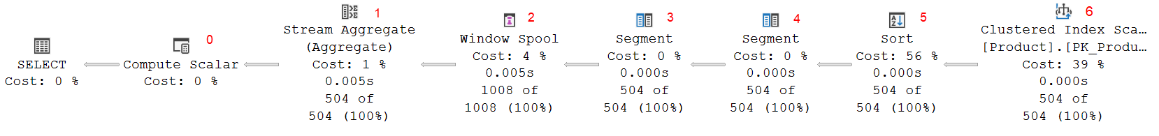
(Click on the picture to enlarge)

Some things are the same as in the previous examples. The right hand side is still a Clustered Index Scan, to get all rows, and then a Sort, to order them by ProductLine and ListPrice. And on the left hand side, we still see a Window Spool, to replay the visible window frame for each row, a Stream Aggregate, to aggregate the rows from that replayed frame into a single row, and a Compute Scalar, to handle the (theoretical, but in this specific case impossible) case of a zero-row window frame.

But the middle looks different. There is no Sequence Project to compute the row number within the partition for each row. Nor a Compute Scalar to compute the top and/or bottom row number of the current frame. Instead, there are now two Segment operators, instead of the one we used to see. Segment #4 is familiar. Just as in the other execution plans we have seen so far, this operator sets Segment1004 to indicate when a new partition (window) starts, because the ProductLine column changes.

Segment #3 is unique for this execution plan. It adds a second segment column, Segment1005. And this segment column is based on a change in any of ProductLine and ListPrice. So this second segment column marks a new segment whenever the first marks a new segment, but it also marks a new segment when the ProductLine remains the same, but ListPrice changes. In other words, each segment marked by this operator is a set of rows that all have the same PARTITION BY value as well as the same ORDER BY value. So for the RANGE specification, all rows in the current segment need to be included in the aggregation to get the correct value.

The Window Spool operator can then use these segment columns to replay the correct rows to the Stream Aggregate operator. Let’s say that one of the partitions has four rows, and the values in the ORDER BY column are 1, 1, 2, and 2. Segment1004 will be set on only the first of these rows, and cause Window Spool to empty its worktable. It then reads ahead to find all other rows in the same segment as indicated by the second segment column, Segment1005, which is set on both the first and the third row. Then it returns the first row as the current row, followed by the rows in its frame, the first and second rows. After that, it returns the second row, once more followed by that same frame. The third row has Segent1005 set, so now it once more reads ahead, and then returns that third row as the current row, followed by the entire frame (rows 1 to 4). And then, finally, it returns the fourth row and once more that same frame.

Except … it actually doesn’t. Since we start at UNBOUNDED PRECEDING, the fast-track optimization that we saw before can be applied here as well. So with this optimization, the actual rows returned for the example above are: First row as current row, plus rows one and two to be added to the (at that point empty) frame. Second row as current row, followed by nothing (because the frame remains unchanged). Third row as current row, followed by rows three and four to be added to the frame. And then the fourth row as the current row, followed, once more, by nothing. Just as with ROWS BETWEEN UNBOUNDED PRECEDING AND CURRENT ROW, we end up returning each row twice, once as current row and once as a row to be added to the running aggregate. Just in slightly different order.

The Window Spool operator has to store all rows within the same (secondary) segment in its work table. Though unlikely, it is always possible that there are more than 10,000 rows with the same values in both the PARTITION BY and the ORDER BY columns. Hence, this worktable is always stored on disk, never in memory.

It is extremely important to always specify ROWS instead of RANGE if you don’t need the RANGE functionality. If you need normal running aggregates, and you accidentally specify RANGE, then you will hopefully notice your error when you run tests and see the invalid results returned for rows that have the same value in the ORDER BY column(s). But there is one nasty exception. When the ORDER BY column happens to have only unique values, then ROWS and RANGE by definition return the same results. So no amount of testing will reveal if you accidentally used RANGE instead of ROWS. But there still IS a difference in performance. For the two queries below, the first will store the worktable in memory, while the second stores it on disk. That causes almost 190,000 logical reads, and on my laptop, the second query takes about twice as long as the first, and takes four times as much CPU time.

SELECT soh.SalesOrderID,
       SUM(soh.TotalDue) OVER (ORDER BY soh.SalesOrderID
                               ROWS BETWEEN UNBOUNDED PRECEDING
                                        AND CURRENT ROW) AS RunTotal
FROM Sales.SalesOrderHeader AS soh;

SELECT soh.SalesOrderID,
       SUM(soh.TotalDue) OVER (ORDER BY soh.SalesOrderID
                               RANGE BETWEEN UNBOUNDED PRECEDING
                                         AND CURRENT ROW) AS RunTotal
FROM Sales.SalesOrderHeader AS soh;

Unfortunately, the OVER clause provides what might at first seem to be a very handy default, that can save a lot of typing. If you specify an ORDER BY, but do not also specify the frame, then it will default to a running aggregate, such as in the query below:

SELECT soh.SalesOrderID,
       SUM(soh.TotalDue) OVER (ORDER BY soh.SalesOrderID) AS RunTotal
FROM Sales.SalesOrderHeader AS soh;

But the sad news is that this default is actually defined as RANGE BETWEEN UNBOUNDED PRECEDING AND CURRENT ROW. Not ROWS. Which in the case of the example above returns the same results, but at a much worse performance. And if there are actually duplicates in the ORDER BY column, then the default is most likely not what you want!

So, bottom line: always specify the ROWS or RANGE expression explicitly!

RANGE BETWEEN CURRENT ROW AND CURRENT ROW

The specification BETWEEN CURRENT ROW AND CURRENT ROW may appear weird at first. And, most of all, totally redundant. And that is indeed correct … when talking about a ROWS specification. ROWS BETWEEN CURRENT ROW AND CURRENT ROW literally means the current row only, and an aggregation of just the current row will just return the current row. (For the record, the optimizer does not recognize the insanity of such a query as it is, and will happily introduce all the overhead to make it replay and aggregate single-row window frames. So don’t do this, please.)

But RANGE BETWEEN CURRENT ROW AND CURRENT ROW actually makes more sense. As already explained, with RANGE, an upper bound of CURRENT ROW does not always end at the current row, but at the last row with the same ORDER BY value. Similarly, a lower bound of CURRENT ROW means it starts at the first row with the same ORDER BY value. Which in effect means that, for every row in a partition with a specific value in the ORDER BY column(s), the window frame includes all rows with those same ORDER BY value(s).

That still does not mean that RANGE BETWEEN CURRENT ROW AND CURRENT ROW is really actually useful. You can just move the ORDER BY column(s) to the PARTITION BY clause and remove the frame, to get the exact same results. So the two queries below are effectively the same:

SELECT p.ProductID,
       p.Name,
       p.ListPrice,
       p.ProductLine,
       SUM (p.ListPrice) OVER (PARTITION BY p.ProductLine
                               ORDER BY p.ListPrice
                               RANGE BETWEEN CURRENT ROW
                                         AND CURRENT ROW) AS SumWithRange
FROM   Production.Product AS p;

SELECT p.ProductID,
       p.Name,
       p.ListPrice,
       p.ProductLine,
       SUM (p.ListPrice) OVER (PARTITION BY p.ProductLine,
                                            p.ListPrice) AS SumWithRange
FROM   Production.Product AS p;

And indeed, the execution plan for the first is the same as the execution plan for the second, using the pattern we have already seen before, multiple times, for aggregates on a window without any frame. Except that in this case the window boundaries are determined by the combination of two columns, and not a single one. (You only see this as a real difference in the Group By property of the Segment operator).

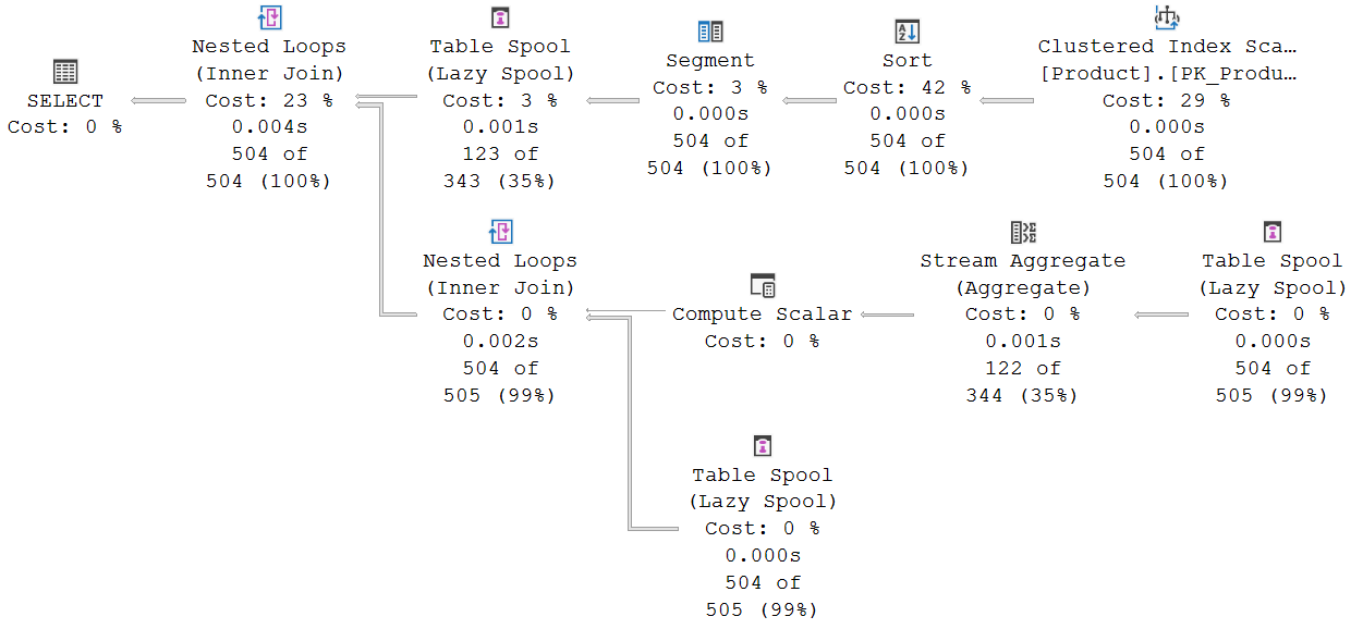
(Click on the picture to enlarge)

Summary

The number of possible RANGE specifications is by itself already limited. And most do not even need support in the execution plan. Some can be converted into an equivalent query that uses a frameless window. Only two cannot, and they are each other’s reverse. Hence, execution plans only have direct support for RANGE BETWEEN UNBOUNDED PRECEDING AND CURRENT ROW. This returns the same as the similar ROWS specification in cases where the combination of PARTITION BY and ORDER BY columns cannot have duplicate values, but at a huge performance hit. When it is possible to have duplicate values, then the results are not the same, and you need to choose the one that is right for your case.

When you use an OVER clause with ORDER BY but without specifying a frame, then the default frame of RANGE BETWEEN UNBOUNDED PRECEDING AND CURRENT ROW applies, with its (probably unwanted) performance hit.

This concludes the coverage of the OVER clause with aggregation. But it does not complete this mini-series on window functions. In the next episode, I’ll turn my attention to the LAG and LEAD functions, and explain how they are actually just a special case of aggregation with a window frame.

As always, please let me know if there is any execution plan related topic you want to see explained in a future plansplaining post and I’ll add it to my to-do list!