This is part twenty-seven of the plansplaining series, and episode five in the mini-series on window functions. The previous parts covered the basics, fast-track optimization, window frames ending at UNBOUNDED FOLLOWING, and window frames specified with RANGE instead of ROWS.

In this post, we will shift our attention to the LAG and LEAD functions. Two functions that do not even accept a window frame specification. So why are they in this series? Read on to find out!

LAG

LAG and LEAD were introduced in SQL Server 2012. They require an OVER clause, but it can only specify PARTITION BY and ORDER BY. No ROWS / RANGE specification for a window frame. Which makes them the stand out as unusual in this series.

By default, they return a value from the last row before the current row, or from the first row after the current row, based on the specified sort order and while observing the specified partition boundaries. But there are two optional parameters, an offset to specify that you want, for instance, the third-last row or the second-next row. And the default parameter specifies a value to be used instead of NULL when the indicated row falls outside of the partition.

So, let’s look at an example.

SELECT p.ProductID,
       p.Name,
       p.ListPrice,
       p.ProductLine,
       LAG (p.ListPrice,2,12.34) OVER (PARTITION BY p.ProductLine
                                       ORDER BY p.ListPrice) AS EarlierPrice
FROM   Production.Product AS p;

Here is the execution plan for the query above.

(Click on the picture to enlarge)

I probably could have just reused one of the older screenshots because (apart from one single value) there is no visible difference between this execution plan and many of the plans we have seen in the previous posts. This totally looks like an execution plan for aggregation of a framed window. And that is because it is an execution plan for aggregation of a framed window.

The devil is, as always, in the details. And the most important details can in this case be found in the two Compute Scalar operators, and in the Stream Aggregate.

The right-most Compute Scalar computes, as we have seen before in these execution plans, both the top row number and the bottom row number. And they are both computed as the same value: row number minus 2. So apparently, we are applying a framed window that could be specified as ROWS BETWEEN 2 PRECEDING AND 2 PRECEDING. A frame that is always just a single row, the row that is two rows before the current row. Which is of course the row we want to return values from in our LAG expression, since the optional second parameter is 2.

So we now know that Window Spool will, for each row, return first the current row and then all rows in that single-row window frame that starts and ends two rows prior. Stream Aggregate then, as always when its child is a Window Spool, uses the first row only to set initial values but excludes it from the aggregation, and then aggregates the other rows. In this case just one. So there is no actual aggregation going on in this case, but we still do need this operator to condense each set of “current row + rows in frame” to “single row including aggregation results”.

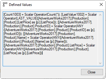As you can see on the right, most of the columns returned are just the columns from the current row, that are needed for the SELECT list. These are produced by the ANY aggregate function. But there are also two new columns. Count1003 is simply a count of the rows in the window. You might think this is always 1 and hence superfluous, but you’ll see in a bit that this is not always the case. The other new column is called LastValue1002, and is computed using the LAST_VALUE aggregate function, which directly equates to the T-SQL aggregate function LAST_VALUE. During accumulation of the input data in Stream Aggregate, this function simply always sets the internal counter to the value from the current row. For the record, since the number of rows to aggregate is always 1, SQL Server could just as well have chosen almost any other aggregate function.

The final step is the leftmost Compute Scalar. Here we see how the Count1003 and LastValue1002 columns are used to determine the final result. A CASE expression tests whether the number of rows in the single row frame is 0. But why? Well, that is because the single row frame might also be an empty frame. For the first and second row in each partition, there is no row that is two rows prior, so Window Spool returns the current row and then nothing, and Stream Aggregate returns the results after initialization: 0 in Count1003 and NULL in LastValue1002. This Defined Values replaces that NULL with the specified default of 12.34. Note that we cannot simply test on a NULL in LastValue1002: the third parameter of LAG only applies when the indicated row does not exist in the partition, we still expect a NULL in the results if, two rows before the current row, ListPrice happens to be NULL. Also note that, if you omit the default parameter, the execution plan will not include this Compute Scalar and also not compute the Count1002 column; the NULL returned by Stream Aggregate for LAST_VALUE when there are no rows to aggregate is already the desired result in this case, so no extra work is needed.

So effectively, we can conclude that a query that uses LAG without default is effectively just converted to the exact equivalent query that uses LAST_VALUE on a single-row window frame, as follows:

SELECT p.ProductID,
       p.Name,
       p.ListPrice,
       p.ProductLine,
       LAG (p.ListPrice,2) OVER (PARTITION BY p.ProductLine
                                 ORDER BY p.ListPrice) AS EarlierPrice
FROM   Production.Product AS p;

SELECT p.ProductID,
       p.Name,
       p.ListPrice,
       p.ProductLine,
       LAST_VALUE(p.ListPrice) OVER (PARTITION BY p.ProductLine
                                     ORDER BY p.ListPrice
                                     ROWS BETWEEN 2 PRECEDING
                                              AND 2 PRECEDING) AS EarlierPrice
FROM   Production.Product AS p;

Add the default parameter, and a bit of extra logic is added that, though simple to explain and implement, is actually quite verbose in SQL Server:

SELECT p.ProductID,
       p.Name,
       p.ListPrice,
       p.ProductLine,
       LAG (p.ListPrice,2,12.34) OVER (PARTITION BY p.ProductLine
                                       ORDER BY p.ListPrice) AS EarlierPrice
FROM   Production.Product AS p;

SELECT p.ProductID,
       p.Name,
       p.ListPrice,
       p.ProductLine,
       CASE WHEN COUNT_BIG(*) OVER (PARTITION BY p.ProductLine
                                    ORDER BY p.ListPrice
                                    ROWS BETWEEN 2 PRECEDING
                                             AND 2 PRECEDING) = 0
            THEN CAST(12.34 AS money)
            ELSE LAST_VALUE(p.ListPrice) OVER (PARTITION BY p.ProductLine
                                               ORDER BY p.ListPrice
                                               ROWS BETWEEN 2 PRECEDING
                                                        AND 2 PRECEDING)
       END AS EarlierPrice
FROM   Production.Product AS p;

-- A bit shorter and easier to understand with the new (SQL2022) named window feature.
SELECT p.ProductID,
       p.Name,
       p.ListPrice,
       p.ProductLine,
       CASE WHEN COUNT_BIG(*) OVER MyWindow = 0
            THEN CAST(12.34 AS money)
            ELSE LAST_VALUE(p.ListPrice) OVER MyWindow
       END AS EarlierPrice
FROM   Production.Product AS p
WINDOW MyWindow AS (PARTITION BY p.ProductLine
                    ORDER BY p.ListPrice
                    ROWS BETWEEN 2 PRECEDING
                             AND 2 PRECEDING);

LEAD

If you change LAG to LEAD in any of the previous examples, you get basically the same execution plan. The only difference is that now the top row number and bottom row number of the window frame are computed as the current row number minus rather than plus the value of the second parameter (or 1 if no second parameter is given).

So once more, the following transformation is made internally (in case there is no default specified), and then an execution plan with the standard pattern for framed window aggregates is used:

SELECT p.ProductID,
       p.Name,
       p.ListPrice,
       p.ProductLine,
       LEAD (p.ListPrice,2) OVER (PARTITION BY p.ProductLine
                                  ORDER BY p.ListPrice) AS LaterPrice
FROM   Production.Product AS p;

SELECT p.ProductID,
       p.Name,
       p.ListPrice,
       p.ProductLine,
       LAST_VALUE(p.ListPrice) OVER (PARTITION BY p.ProductLine
                                     ORDER BY p.ListPrice
                                     ROWS BETWEEN 2 FOLLOWING
                                              AND 2 FOLLOWING) AS LaterPrice
FROM   Production.Product AS p;

New functionality in SQL Server 2022

In SQL Server 2022, Azure SQL Database, and Azure SQL Managed Instance, a new, optional keyword was added to the LAG and LEAD functions: IGNORE NULLS or RESPECT NULLS. When neither is specified, RESPECT NULLS is assumed, which specifies the same behavior as in older versions, as explained above. With IGNORE NULLS, rows with a NULL in the listed column are ignored. Or, well, at least sort of.

To illustrate the difference between the various options, we need to change to another table and query. There are no NULL values in ListPrice, after all. So here is an example that pits all options against each other.

SELECT p.PersonType,
       p.FirstName,
       p.MiddleName,
       p.LastName,
       LAG (p.MiddleName, 2, '-') OVER MyWindow AS NotSpecified,
       LAG (p.MiddleName, 2, '-') RESPECT NULLS
                                  OVER MyWindow AS Respect,
       LAG (p.MiddleName, 2, '-') IGNORE NULLS
                                  OVER MyWindow AS Ignore
FROM   Person.Person AS p
WINDOW MyWindow AS (PARTITION BY p.PersonType
                    ORDER BY p.LastName, p.FirstName);

The NotSpecified and Respect columns are of course always the same, because we already know that RESPECT NULLS is assumed when nothing is specified. But the last column, Ignore, sometimes returns different result. In the picture below, I have pasted together screenshots from various parts of the output, to illustrate all relevant details.

The first difference is in row 14. The LAG function looks back to row 12, which has a NULL MiddleName. With RESPECT NULLS, that does not matter. But with IGNORE NULLS, this row is now ignored and LAG looks back one row further, to row 11. Hence we see another K in the IGNORE column.

The second fragment shows that if there are multiple rows adjacent to each other in the same partition, LAG with IGNORE NULLS will skip past all of them, and effectively carry forward the I from row 240 for as many rows as needed until the LAG function looks back at a row with a non-NULL value.

The last fragment shows an interesting behavior of LAG’s default parameter. Even though rows with a NULL MiddleName need to be ignored, the supplied default value is still only used on the first two rows within the partition for PersonType = ‘GC’. You could say that, logically speaking, LAG first checks whether the target row for LAG is within the partition and uses the default is not, and only after that it ignores the rows with NULL values. Or you could say that the default parameter is not affected by the IGNORE NULLS setting. No matter how you phrase it, the effect is that you still can get NULL results in the Ignore column.

To see how the execution plan is affected by IGNORE_NULLS, let’s simplify the query above so that only that column is left, and then check the execution plan plus run-time statistics.

SELECT p.PersonType,
       p.FirstName,
       p.MiddleName,
       p.LastName,
       LAG (p.MiddleName, 2, '-') IGNORE NULLS
                                  OVER (PARTITION BY p.PersonType
                                        ORDER BY p.LastName, p.FirstName) AS Ignore
FROM   Person.Person AS p;

(Click on the picture to enlarge)

Once more, there are no directly visible differences between this execution plan and all the previous ones. Because, once more, the differences are in the properties only.

The Compute Scalar roughly in the middle of the execution plan still computes the bottom row number as the current row number minus two. But it no longer computes a top row number, and as we have seen in previous posts, that means that we are now working with an effective window frame of ROWS BETWEEN UNBOUNDED PRECEDING AND 2 PRECEDING. No longer the single-frame window we used before. Luckily, since we start at UNBOUNDED PRECEDING, fast-track optimization does apply, so we are not confronted with the huge performance cost that this otherwise could result in!

The Defined Values property of the Stream Aggregate is almost the same as in the execution plan for LAG with RESPECT NULLS (or no NULLS specification). Almost. But not exactly. If you look carefully at the screenshot shown, you will see that the specification for LastValue1002 no longer uses LAST_VALUE, but now uses LAST_VALUE_IGNORE_NULLS, a new aggregate function that was introduced in SQL Server 2022, and that can only be used internally. You cannot use this function in T-SQL yourself. (But you can use LAST_VALUE with the IGNORE NULLS option to get the same effect).

While LAST_VALUE always replaces the value in the internal counter with the value from the current row, LAST_VALUE_IGNORE_NULLS only does this when the current value is not NULL. Otherwise it leaves the internal counter unchanged, which causes exactly the carry forward effect we saw in the sample results above.

The Compute Scalar then does the exact same as we have seen before. It checks whether a row that is two rows before the current row even exists at all in the partition, by checking the Count(*) of the rows in the frame that Window Spool returned to Stream Aggregate. Note that this is now not the number of rows in the frame ROWS BETWEEN 2 PRECEDING AND 2 PRECEDING, but in the frame ROWS BETWEEN UNBOUNDED PRECEDING AND 2 PRECEDING. But that difference is not important in this context; for rows that are at one or two rows past a partition boundary, both are 0; for rows that are further beyond a boundary, both are more than 0.

Also note that, if the formula for Count1003 had been changed to use COUNT(p.MiddleName) instead of Count(*), then the supplied default of ‘-‘ would have applied to rows 276 – 279 in the sample output above as well, effectively making the default parameter respect the IGNORE NULLS setting as well. However, since the documentation states that this value is only returned when the specified offset is beyond the scope of the partition, that would have been incorrect. (One can argue which would be the more desired behavior, but that is beyond the scope of this post).

LEAD with IGNORE NULLS

Of course, the IGNORE NULLS and RESPECT NULLS clauses can be applied to LEAD as well, with the same effect. It is, however, important to realize that, where LAG looks back at even earlier rows when a row with a NULL is ignored, LEAD doesn’t look back but instead looks forward, as you can see in the query and output below:

SELECT p.PersonType,
       p.FirstName,
       p.MiddleName,
       p.LastName,
       LEAD (p.MiddleName, 2, '-') RESPECT NULLS
                                   OVER MyWindow AS Respect,
       LEAD (p.MiddleName, 2, '-') IGNORE NULLS
                                   OVER MyWindow AS Ignore
FROM   Person.Person AS p
WINDOW MyWindow AS (PARTITION BY p.PersonType
                    ORDER BY p.LastName, p.FirstName)
ORDER BY p.PersonType, p.LastName, p.FirstName;

Rows 239 and 240 look at rows 241 and 242 for the LEAD. But those rows have a NULL MiddleName, and the IGNORE NULLS option forces to look, not at the last row before those (240, with MiddleName I), but at the next row after (243, MiddleName A). So instead of the carry forward we had with LAG, we now effectively have a carry backward of this A.

Let’s once more reduce the query to have only the single LEAD with IGNORE NULLS, to focus on how this is processed. To reduce the complexity a bit further, I have also removed the default parameter. We already know how SQL Server handles this and do not need to repeat it in each next sample. The last modification is a hint to prevent parallelism, again to keep the execution plan a bit simpler.

SELECT p.PersonType,
       p.FirstName,
       p.MiddleName,
       p.LastName,
       LEAD (p.MiddleName, 2, '-') IGNORE NULLS
                                   OVER MyWindow AS Ignore
FROM   Person.Person AS p
WINDOW MyWindow AS (PARTITION BY p.PersonType
                    ORDER BY p.LastName, p.FirstName)
ORDER BY p.PersonType, p.LastName, p.FirstName
OPTION (MAXDOP 1);

Before showing the execution plan, let’s first discuss what to expect. The trick we used above, to simply start the frame at UNBOUNDED PRECEDING instead of 2 FOLLOWING, and still end at 2 FOLLOWING, does not work. We already saw that the value we need might be from 3 or 4 rows after the current row, or even more. So we need an end point of UNBOUDED FOLLOWING. And we also don’t actually need any rows before the LEAD target row, so the start of the frame can be back to 2 FOLLOWING. And, finally, with that changed window frame, we now also need to make sure to use the internal aggregate function FIRST_VALUE_IGNORE_NULLS (which already exists since SQL Server 2012) instead of LAST_VALUE_IGNORE_NULLS. So we have basically converted the LEAD function with IGNORE NULLS from the query above to this equivalent query (using FIRST_VALUE with the IGNORE NULLS clause, because FIRST_VALUE_IGNORE_NULLS cannot be used directly in T-SQL):

SELECT p.PersonType,
       p.FirstName,
       p.MiddleName,
       p.LastName,
       FIRST_VALUE(p.MiddleName) IGNORE NULLS
                                 OVER (PARTITION BY p.PersonType
                                       ORDER BY p.LastName, p.FirstName
                                       ROWS BETWEEN 2 FOLLOWING
                                                AND UNBOUNDED FOLLOWING) AS Ignore
FROM   Person.Person AS p
ORDER BY p.PersonType, p.LastName, p.FirstName
OPTION (MAXDOP 1);

Both the query with LEAD as well as the equivalent rewrite with FIRST_VALUE result in the exact same execution plan:

(Click on the picture to enlarge)

Now, if you look at this execution plan in SSMS instead of at the screenshot here, you might start to notice lots of little and not-so-little things that do not match the query above. But then you will, hopefully, recall what we learned in the previous part where we discussed window frames ending at UNBOUNDED FOLLOWING. This is such a window frame, so, as explained in that post, SQL Server reverses the sort order of the frame specification, makes the corresponding changes to the frame specification, and in this case also changes the order-sensitive function FIRST_VALUE to LAST_VALUE. So you might say that the query above goes through yet another transformation step, to look like this:

SELECT p.PersonType,
       p.FirstName,
       p.MiddleName,
       p.LastName,
       LAST_VALUE(p.MiddleName) IGNORE NULLS
                                OVER (PARTITION BY p.PersonType
                                      ORDER BY p.LastName DESC, p.FirstName DESC
                                      ROWS BETWEEN UNBOUNDED PRECEDING
                                               AND 2 PRECEDING) AS Ignore
FROM   Person.Person AS p
ORDER BY p.PersonType, p.LastName, p.FirstName
OPTION (MAXDOP 1);

And now you will indeed see that all the elements in the execution plan nicely line up to the elements in the query above.

(Note that in reality, SQL Server does not actually do any such transformations on the actual query text. They are applied on internal structures such as the parse tree, the query tree, and the memo.)

Performance alert

Because of the above, the introduction of the IGNORE NULLS option can result in very unexpected performance deterioration. Let’s look at a query that was valid before SQL Server 2022, so with no specification:

SELECT p.PersonType,
       p.FirstName,
       p.MiddleName,
       p.LastName,
       LAG (p.MiddleName)  OVER MyWindow AS WithLag,
       LEAD (p.MiddleName) OVER MyWindow AS WithLead
FROM   Person.Person AS p
WINDOW MyWindow AS (PARTITION BY p.PersonType
                    ORDER BY p.LastName, p.FirstName)
ORDER BY p.PersonType, p.LastName, p.FirstName;

This is processed quite effectively. LAG and LEAD are converted to different frame specifications, but with the same partitioning and the same sort order. So there is just a single Sort operator in the execution plan. And that is because there is no index that we can read from to get the data in the order we need it, otherwise there would have been no Sort at all.

But if we add the IGNORE NULLS option, our performance drops deep!

SELECT p.PersonType,
       p.FirstName,
       p.MiddleName,
       p.LastName,
       LAG (p.MiddleName)  IGNORE NULLS OVER MyWindow AS WithLag,
       LEAD (p.MiddleName) IGNORE NULLS OVER MyWindow AS WithLead
FROM   Person.Person AS p
WINDOW MyWindow AS (PARTITION BY p.PersonType
                    ORDER BY p.LastName, p.FirstName)
ORDER BY p.PersonType, p.LastName, p.FirstName;

All of a sudden one of the two functions is converted into something with UNBOUNDED FOLLOWING, which then results in a reversed sort order. And for that we need extra Sort operators. The execution plan for the query above uses three Sort operators rather than just one, and this bumps the estimated plan cost even above the default threshold for parallelism, so that a parallel execution plan is generated.

By the way, simply reversing the order in which the LAG and LEAD columns are specified in the SELECT list reduces the amount of Sort operators from three to two. Still more than without IGNORE NULLS, but at least not as much as the first version of the query. This is effectively the same bad optimizer choice issue that I already mentioned in an earlier part of this series, and that I created this feedback item for.

Summary

When a query uses LAG or LEAD, it is internally converted into an equivalent expression that uses framed window aggregates on a single window frame. On SQL Server 2022 and in Azure, you can add IGNORE NULLS to change how NULL values are handled, and then the execution plan uses a window frame that starts at the partition boundary, with fast-track optimization. Both are very fast. But beware that for specifically LEAD with IGNORE NULLS, the sort order has to be reversed to process the windowed aggregation.

We are now almost at the end of the mini-series on window functions, that was ultimately all kicked off by a T-SQL Tuesday challenge. When I saw that challenge, I had expected to cover window functions in a single post. It grew to this collection of five, and most are actually quite long! But we are nearly there now. I have just one post left, and that should be a much shorter one. So please join me next time, for the curious case of the missing FIRST_VALUE function.

As always, please let me know if there is any execution plan related topic you want to see explained in a future plansplaining post and I’ll add it to my to-do list!