I had to skip three months, but finally it is here: part eight of the plansplaining series. Each of these posts takes an execution plan with an interesting pattern, and details exactly how that plan works.

I am pretty sure that (almost) everyone reading this blog knows that a CTE (Common Table Expression) is an independent subquery that can be named and then referenced (multiple times if needed) in the main query. This makes CTEs an invaluable tool to increase the readability of complex queries. Almost everything we can do with a CTE can equally well be done by using subqueries directly in the query but at the cost of losing readability.

However, there is also one feature that is actually unique to CTEs: recursion. This blog post is not about what this feature is, what it does, or how to write the code. A brief description is given as part of the complete explanation of CTEs in Books Online, and many bloggers have written about recursive CTEs as well.

For this post, I’ll assume the reader knows what a recursive CTE is, and jump into the execution plan to learn how this recursion is actually implemented.

Sample query

The query below is modified from one of the examples in Books Online. This query can be executed in any version of the AdventureWorks sample database. It returns the exploded Bill of Materials for the “Road-550-W Yellow, 44” bicycle (which has ProductID 800).

WITH Parts
  AS (SELECT      b.ProductAssemblyID, b.ComponentID, b.PerAssemblyQty, 1 AS Lvl
      FROM        Production.BillOfMaterials AS b
      WHERE       b.ProductAssemblyID = 800
      AND         b.EndDate IS NULL
      UNION ALL
      SELECT      b.ProductAssemblyID, b.ComponentID, b.PerAssemblyQty, p.Lvl + 1
      FROM        Production.BillOfMaterials AS b
      INNER JOIN  Parts                      AS p
            ON    b.ProductAssemblyID = p.ComponentID
            AND   b.EndDate IS NULL)
SELECT  Parts.ProductAssemblyID, Parts.ComponentID, Parts.PerAssemblyQty, Parts.Lvl
FROM    Parts;

The execution plan for this query is quite complex, as you can see below. (As in earlier episodes, I have added the NodeID numbers into the execution plan to make it easier to reference individual operators).

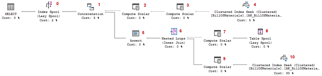
This execution plan does several things that are fairly easy to understand. And then there is some other, much more interesting stuff to make the magic of recursion happen. To prevent this post from becoming too long, I will describe the simpler parts very briefly. Feel free to run this query on your own system to dive deeper in the parts I skip. Make sure you understand them, and don’t hesitate to leave a question in the comments section if anything is unclear to you!

The top line

As always, execution of the query starts of the top left with operators calling their child operator (from the first input in the case of Concatenation #1), until Clustered Index Seek #4 is invoked. The properties of this operator show that it uses an index on (ProductAssemblyID, ComponentID, StartDate) to quickly find all rows that match the predicate of the anchor query. It processes them in order of ascending ComponentID, returning the three columns from this table that are used in the query.

As always, it is important to remember that an operator never just returns all rows; it waits until it is called, does the work needed to produce and return the next row, and then saves state and halts until it is called again. In this case we will see that the operators on the top row of the execution plan keep calling each other until all matching rows are processed so it not especially relevant in this case but it’s still important to always be aware of this!

Compute Scalar #3 receives rows from Clustered Index Seek #4. It adds one extra column, named Expr1001, that is always set to 1 (one). We will later see that this Expr1001 column will eventually be returned to the client as the Lvl column; the fixed value of 1 in this operator confirms what we already suspected, that the top line evaluates the anchor query.

Compute Scalar #2 then adds yet another column, Expr1012, that is 0 (zero). We will later see what this column is used for.

The rows are then returned to Concatenation #1, which implements the UNION ALL expression in the query. Like any Concatenation operator, it simply reads rows from its first input and returns them unchanged. Once the first input is exhausted it moves to the second input (which I will discuss further down). Concatenation operators can have more than two inputs, but in this execution plan it has just two.

A side effect of a Concatenation operator in an execution plan is that it renames all columns, which can make it harder to follow what is going on. I often end up writing down the column names in a file on a second monitor, or just on a simple scrap of paper. In this case, the most important thing to remember is that the “new” column Expr1015 refers to the original Expr1012 (from Compute Scalar #2) for rows from the first input, and Expr1014 for the second input.

The other four columns, Recr1008 to Recr1011, correspond to the four columns returned by the query.

Index Spool #0

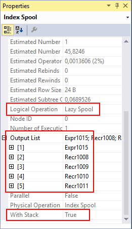The final operator on the top line of the execution plan is Index Spool #0. Looking at its properties we see that the With Stack property is True, which means that this is actually a “stack spool”. As you can see in the description of this processing type on the Index Spool page in the Execution Plan Reference, this means that it uses a worktable indexed by the first column in the Column List, which supposedly represents the recursion level. This is Expr1015, originating from Expr1012 and always zero for the top line – this bit will get more interesting later on. For now, because all rows have the same value the engine will add a uniqueifier to each row in the worktable to ensure uniqueness and to guarantee that rows can be retrieved in the correct order.

The logical operation is Lazy Spool; this means that it returns its input rows immediately, after storing them in the worktable.

The Output List property says that all five columns returned by Concatenation #1 are stored in the worktable and returned to the calling operator. However we know from the query and its results that only the four columns Recr1008 to Recr1011 are actually returned to the client; Expr1015 is not and is apparently filtered out in the top-left SELECT operator, though this is not exposed in the execution plan.

This construction is due to a limitation of the Index Scan operator: the Output List property defines both the structure of the worktable and the columns returned. In this case the Expr1015 column is not needed by any parent of the operator and hence doesn’t need to be in the output. But it IS needed in the worktable (we’ll see why further down), and hence needs to be in the Output List property.

Top line condensed

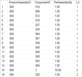
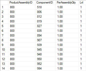Taking all the operators of the top line together, we can see that each call goes all the way from SELECT to Clustered Index Seek #4, which reads and returns a row that then propagates all the way back to SELECT and to the client. This process repeats a total of 14 times, reading and returning the 14-row result set of the anchor part of the recursive CTE. If we could pause execution at this time we would see a result set as shown to the right.

The worktable created by Index Spool #0 contains these same rows at this point, but with two additional columns: one for Expr1015 (equal to zero for all these rows) and one with a four-byte uniqueifier on all rows except the first, to ensure that the clustered index of the worktable keeps these rows in place. (See this article for more details on the exact internal storage of the various spool types).

After returning the 14^th row the execution once again propagates all the way through to Clustered Index Seek #4, but this time it returns an “end of data” signal because no more rows satisfy the conditions in its Seek Predicates and Predicate properties. The two Compute Scalar operators simply relay this “end of data” signal to their parents. Once Concatenation #1 receives it, it responds by moving to its next input, calling Assert #5.

The bottom part

Most operators when called to return a row start by calling their own child operator for a row. The operators on the second input of Concatenation #1 are no exception, so once Assert #5 is called the first time control immediately passed through Nested Loops #6 and Compute Scalar #7 to Table Spool #8, the second spool operator in this plan.

Table Spool #8

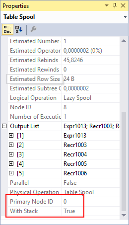Since this Table Spool has no inputs, it must work as a consumer. This is confirmed by seeing the Primary Node ID property that points to Index Spool #0 as the builder of the worktable that is read by this Table Spool. You can also see that the With Stack property set to true (as is expected– a “stack spool” always consists of a builder Index Spool combined with a consumer Table Spool).

The behavior of the Table Spool part of a stack spool combination is to remove the previously read row from the worktable and then read the row with the highest key value. Remember that the key is on the Expr1015 column which is supposed to be the recursion level, and that the system uses an internal uniqueifier to distinguish between duplicates which means that within each Expr1015 value the last added row will have the highest uniqueifier. So by reading the highest key value, the operator effectively reads the most recently added row within the highest recursion level.

You may also note that the column names in the Output List property are different from the column names in the Output List of Index Spool #0 where the worktable is created. This is normal behavior. The columns are matched by order. So for example, the third column listed in the Output List of Index Spool #0 is Recr1009 (which was the name assigned by Concatenation #1 to the ComponentID column from both the first and the second input). The third input listed in Table Spool #8 is Recr1004, so now Recr1004 contains the ComponentID value.

For this first call, there is no previously read row so there is nothing to delete. The operator reads the row with the highest key value – all rows currently in the worktable have Expr1015 equal to zero, so the last added row will be read and returned to the calling operator. This is the row with ComponentID 994.

The join logic

Table Spool #8 passes this row to its parent, Compute Scalar #7. Its Defined Values property shows that this operator computes a new expression, Expr1014, and sets its value to Expr1013 + 1. Since Expr1013 was 0, Expr1014 will be 1.

The modified row is returned to the parent operator (Nested Loops #6). This operator uses the Outer References property to push several values from its outer (top) input into the inner (bottom) input. These values are then used by Clustered Index Seek #10 to quickly find rows with ProductAssemblyID equal to the Recr1004, which we already saw to be the new name for the column holding the ComponentID. The Clustered Index Seek #10 also has a residual Predicate property for the additional filtering on EndDate IS NOT NULL. Based on my knowledge of the data, I expect that for the current Recr1004 value of 994 this Clustered Index Seek #10 will find two rows; on the first call it will return the first of these two matches, a row with ProductAssemblyID 994, ComponentID 3, and PerAssemblyQty 10.00.

This row is passed through Compute Scalar #9, where Expr1007 is computed as Recr1006 + 1; if you are following along with a full mapping of all column names you will realize that this is the computation for the Lvl column in the query. Nested Loops #6 then combines this row with the current row from its outer input and returns the result (to be precise, only the columns that are listed in its Output List property) to its parent operator.

Assert #5

An Assert operator is used in execution plans to check for conditions that require the query to be aborted with an error message. Based on the query you may not have expected to see an Assert in this execution plan, since the query includes nothing that calls for a potential runtime error.

Let’s check the properties of this operator to see if we can find out why it’s there. As you see, it does a simple check on the Expr1014 column: if this column is larger than 100, the query will end with a runtime error. In the current row this column has the value 1 so processing continues. But seeing this condition should help you realize why it’s there: not because of something I included in the query but because of something I omitted. If you are familiar with recursive CTEs, you will know that by default they support a maximum recursion level of 100. This is to prevent us from ourselves – without it, a coding error that results in infinite recursion would cause the query to actually run forever, using more and more resources along the way. The maximum recursion level can be changed, or removed (at your own peril!). If you add the query hint OPTION (MAXRECURSION 0) to the query, the protection is disabled and the Assert operator is removed from the execution plan.

The place of this operator is very important. The check is not done immediately when the new recursion level is computed, but only after they are joined to matching rows from the BillOfMaterials table. This means that if Table Spool #8 reads a row that already has recursion level 100, Compute Scalar will immediately compute the next recursion level at 101, but execution will not stop. First Nested Loops #6 will execute and look for matches. If there are no matches, then it will never return this row with Expr1014 = 101 to its parent operator, Assert #5, and execution will not end with a runtime error. However, when the Nested Loops operator does find a matching row, then  the combined data is returned to Assert #5 and execution stops before this row is ever returned to the client (or even stored in the worktable).

Back to the top

The row that was just produced by the second input of Concatenation #1 is now passed through that operator to Index Spool #0, which adds it to the worktable and then passes it to the client. The fifteenth row of the result set is now added to the data in the results pane of SSMS. This row is in the worktable as well. Because Expr1015 was set to 1 for this row, it is added at the end of the worktable (based on the logical structure imposed by the clustered index – we obviously have no idea and do not care on which page within tempdb this row is stored).

Rinse and repeat

After processing the fifteenth row the operators once more call each other, and this time the call propagates to Nested Loops #6 quickly. But here the path changes. The last thing Nested Loops #6 did was request and return a row from its inner input. It will now do that again, so control is passed through Compute Scalar #9 to Clustered Index Seek #10. The second row with ProductAssemblyID 994 is now read and returned – this is a row with ComponentID equal to 525. This row is then processed exactly the same as the previous row. So at the end, this is the sixteenth row in both the results and the worktable.

If we were to pause execution at this point, the result set would look as shown to the right. The worktable would be equal, though with the addition of Expr1015 (0 for the first fourteen rows, 1 for the last two)) and the hidden uniqueifier to ensure that the rows remain properly ordered.

For the 17^th call the control with pass through the operator in the same way is before. But now Clustered Index Seek #10 finds no more rows to return; its “end of data” signal is relayed trough Compute Scalar #9 to Nested Loops #6, which then requests the next row from its outer (top) input.

This call flows through Compute Scalar #7 to Table Spool #8. As explained above, the Table Spool of a stack spool combination first removes the row it previously read, row 14 in the picture above. After removing this row it then proceeds to fetch the row with the highest key value, which is row 16 in the screenshot above. For this row, Expr1014 is computed as 2 (because it was stored with Expr1015 equal to 1), and then the data is passed to Nested Loops #6. However, since there are no rows in the base table with ComponentID 525, the inner input of this Nested Loops operator returns nothing so Compute Scalar #7 and Table Spool #8 are invoked again.

Now row number 16 in the picture above is removed, since this is the row last processed. After that, the row with the highest key is row 15 in the screenshot, so now this row is passed to Nested Loops #6. And this time it will get matches from its inner (bottom) input, so now more rows will be produced, stored in the worktable (again at the end), and returned to the client.

The same process repeats, over and over again, until all 89 rows of the result set are produced. Over and over again, Table Spool #8 removes the row it read last from the worktable and then reads the row with the highest key value, which is always the row added last. And each time that row actually produces new results in the join, they are added, at the end of the worktable, by Index Spool #0.

Eventually, Table Spool #8 will read the last remaining row from the worktable. After that, either new matches are found and added to the worktable so the process can continue, or no new matches are found. In that last case, Nested Loops #6 will one final time try to get a row from its outer (top) input. Table Spool #8 will remove that final row that it just read, and then see no rows left for it to read and return. It will send an “end of data” signal which then propagates all the way through all operators to the top-left SELECT, and execution of the query stops.

Stack spool

Some of the readers might already be familiar with the concept of a stack. For those who are not, here is a short explanation.

If two elements within a system exchange data and the elements may sometimes produce more data than can be handled immediately, there are two basic structures for exchanging that information: queue-based or stack-based.

The queue-based system, also known as FIFO (“first in first out”) gets its name from the British concept of queueing politely, without elbowing in front of other people. The first to arrive at a bus stop will stand there, the next gets in line behind them, and when the bus arrives the passengers board in the order in which they arrived. A queue within information systems is used to ensure that data is processed in the same order it is produced.

The stack-based system, also known as LIFO (“last in first out”) gets its name from the concept of stacks of plates in a self-service restaurant. When a customer arrives they’ll grab the top plate of the stack. When the dishwasher brings a new plate (or more typical a bunch of new plates) they are simply put on top of the stack. The next customer will grab the plate that was added the most recently. A stack within information systems is used when the data that was added last needs to be processed and removed from the stack first.

Not quite a stack

The combination of an Index Spool and Table Spool, both with the With Stack property set to True, is called a stack spool. That is because it conceptually implements a stack that ports data produced in one part of the execution plan to another part where it is processed. However, it is not a 100% true stack. Official stack implementations would remove a row as it is processed, not after it has been processed and more rows are added. That would be like a restaurant customer adding food to their plate while the dishwasher already stacks now plates upon it, and then the customer will have to get the plate (with the now squashed food) from within the stack while leaving the plates that were added later on top of it.

I am not sure why Microsoft chose to implement this the way it is. After all, it’s probably even easier to build a system that removes the row immediately. However, I do have two theories:

1. Perhaps there are some scenarios with a very complex recursive query where the same row needs to be read multiple times from the same worktable. This is of course not possible if the row is already deleted. However, I have not been able to set up any such scenario; most of my attempts were rejected for violating the rules of recursive CTEs.
2. The more likely explanation is that operators in execution plans are designed to be as efficient as possible, and that one such optimization is that operators that read data from a table (including worktables) do not actually copy the data from the buffer pool to working storage, but just use pointers to the location within the buffer pool. If this were done with data read from the worktable of a stack spool, then deleting that row as it is read would mark that area of the buffer pool as free for reuse – and now there is a risk of other processes overwriting the data when it is still needed.

Conclusion

Recursion may sound like a simple technique, but in reality it rarely isn’t. In this blog post we looked at all the nuts and bolts that come together to implement recursion in the execution plan for a query with a recursive CTE.

The absolute worker bee is the combination of an Index Spool and a Table Spool, both with the With Stack property present and set to true. This combination is also known as a stack spool, because it implements a stack that allows rows to be stored in one place in the plan and then read and processed in another plan using the so-called “LIFO” (last in first out) method. The last row added will always be read and processed first; the first row added will be read last. Understanding this mechanism helps to explain things like, for instance, the order in which rows are returned from a recursive CTE. However, as always, the order of the results in a query is only ever guaranteed if an ORDER BY clause is used – so please don’t go and build logic that relies on the order described in this post. It is subject to change without notice if Microsoft decides to implement a different way to evaluate recursive queries.

But the role of the various Compute Scalar operators should also not be underestimated. In these, the recursion level is computed. It is zero for the anchor query, because no recursion is used in that part. For rows produced in the recursive part, it is set to the recursion level of the input row plus one. We saw this recursion level being used by an Assert operator, to ensure that execution stops when the maximum recursion level is exceeded. But the more important usage of the recursion level is that it defines the clustered index for the worktable. That’s why the computation of the recursion level will not be removed it you disable the maximum recursion check.

I hope to be able to continue this series. Whether the next episode will be ready within a month, I do not know. But I will work on it. However, I am starting to run out of ideas. There are still some notes on my shortlist but I do need reader input here as well! If you see an unusual and interesting pattern in an execution plan, let me know so I can perhaps use it in a future post!