Welcome to part twenty of the plansplaining series. It has been a long time since I last wrote a plansplaining post, partly because of my health, but also for a large part because I was out of ideas. But recently I decided to dig a bit deeper into a feature that was released in SQL Server 2017 and that I had so far not played with: SQL Graph.

SQL Graph is the name for a set of features, introduced in SQL Server 2017 and extended in SQL Server 2019, that bring graph database functionality into SQL Server. See here for the full documentation as provided by Microsoft. In this first post about SQL Graph, I’ll look at what execution plans reveal about the internal structure of graph tables. I’ll then use that knowledge in later parts, where I’ll discuss more advanced queries on graph tables.

Sample data

For my experiments with graph tables, I decided to simply use the sample tables and data that Microsoft has included in their documentation. You can find the script to create and populate the tables here. For your convenience, I have copied the script (cleaned up and reformatted) below.

-- Create a graph demo database
IF NOT EXISTS (SELECT * FROM sys.databases WHERE name = 'GraphDemo')
    CREATE DATABASE GraphDemo;
GO

USE GraphDemo;
GO

-- Create node tables
CREATE TABLE dbo.Person
    (ID   integer PRIMARY KEY,
     name varchar(100)) AS NODE;
CREATE TABLE dbo.Restaurant
    (ID   integer NOT NULL,
     name varchar(100),
     city varchar(100)) AS NODE;
CREATE TABLE dbo.City
    (ID        integer PRIMARY KEY,
     name      varchar(100),
     stateName varchar(100)) AS NODE;

-- Create edge tables.
CREATE TABLE dbo.likes
    (rating integer) AS EDGE;
CREATE TABLE dbo.friendOf AS EDGE;
CREATE TABLE dbo.livesIn AS EDGE;
CREATE TABLE dbo.locatedIn AS EDGE;

-- Insert data into node tables.
INSERT INTO dbo.Person (ID, name)
VALUES (1, 'John'),
       (2, 'Mary'),
       (3, 'Alice'),
       (4, 'Jacob'),
       (5, 'Julie');

INSERT INTO dbo.Restaurant (ID, name, city)
VALUES (1, 'Taco Dell', 'Bellevue'),
       (2, 'Ginger and Spice', 'Seattle'),
       (3, 'Noodle Land', 'Redmond');

INSERT INTO dbo.City (ID, name, stateName)
VALUES (1, 'Bellevue', 'WA'),
       (2, 'Seattle', 'WA'),
       (3, 'Redmond', 'WA');

-- Insert into edge table. While inserting into an edge table,
-- you need to provide the $node_id from $from_id and $to_id columns.
/* Insert which restaurants each person likes */
INSERT INTO dbo.likes
VALUES ((SELECT $node_id FROM dbo.Person WHERE ID = 1),
        (SELECT $node_id FROM dbo.Restaurant WHERE ID = 1), 9),
       ((SELECT $node_id FROM dbo.Person WHERE ID = 2),
        (SELECT $node_id FROM dbo.Restaurant WHERE ID = 2), 9),
       ((SELECT $node_id FROM dbo.Person WHERE ID = 3),
        (SELECT $node_id FROM dbo.Restaurant WHERE ID = 3), 9),
       ((SELECT $node_id FROM dbo.Person WHERE ID = 4),
        (SELECT $node_id FROM dbo.Restaurant WHERE ID = 3), 9),
       ((SELECT $node_id FROM dbo.Person WHERE ID = 5),
        (SELECT $node_id FROM dbo.Restaurant WHERE ID = 3), 9);

/* Associate in which city live each person*/
INSERT INTO dbo.livesIn
VALUES ((SELECT $node_id FROM dbo.Person WHERE ID = 1),
        (SELECT $node_id FROM dbo.City WHERE ID = 1)),
       ((SELECT $node_id FROM dbo.Person WHERE ID = 2),
        (SELECT $node_id FROM dbo.City WHERE ID = 2)),
       ((SELECT $node_id FROM dbo.Person WHERE ID = 3),
        (SELECT $node_id FROM dbo.City WHERE ID = 3)),
       ((SELECT $node_id FROM dbo.Person WHERE ID = 4),
        (SELECT $node_id FROM dbo.City WHERE ID = 3)),
       ((SELECT $node_id FROM dbo.Person WHERE ID = 5),
        (SELECT $node_id FROM dbo.City WHERE ID = 1));

/* Insert data where the restaurants are located */
INSERT INTO dbo.locatedIn
VALUES ((SELECT $node_id FROM dbo.Restaurant WHERE ID = 1),
        (SELECT $node_id FROM dbo.City WHERE ID = 1)),
       ((SELECT $node_id FROM dbo.Restaurant WHERE ID = 2),
        (SELECT $node_id FROM dbo.City WHERE ID = 2)),
       ((SELECT $node_id FROM dbo.Restaurant WHERE ID = 3),
        (SELECT $node_id FROM dbo.City WHERE ID = 3));

/* Insert data into the friendOf edge */
INSERT INTO dbo.friendOf
VALUES ((SELECT $node_id FROM dbo.Person WHERE ID = 1),
        (SELECT $node_id FROM dbo.Person WHERE ID = 2)),
       ((SELECT $node_id FROM dbo.Person WHERE ID = 2),
        (SELECT $node_id FROM dbo.Person WHERE ID = 3)),
       ((SELECT $node_id FROM dbo.Person WHERE ID = 3),
        (SELECT $node_id FROM dbo.Person WHERE ID = 1)),
       ((SELECT $node_id FROM dbo.Person WHERE ID = 4),
        (SELECT $node_id FROM dbo.Person WHERE ID = 2)),
       ((SELECT $node_id FROM dbo.Person WHERE ID = 5),
        (SELECT $node_id FROM dbo.Person WHERE ID = 4));
GO

Internals of a node table

When I first looked at execution plans for graph queries, I noticed that they use columns in the node and edge tables that I myself can’t access. Apparently, the internal format is not the same as what we see when we look at those tables. Some of those differences are very visible. Others are more hidden and harder to figure out. So let’s start there.

Let’s first look at a node table, for instance at dbo.Person. In the script above, it is created with just two columns: ID and name. But when I use SELECT * to query its data, you’ll see that SQL Server actually created a third column.

SELECT *
FROM   dbo.Person AS p;

Here are the results when I ran this on my system:

The result set does not only include the expected ID and name columns, but also one extra column, named $node_id_ followed by 32 hexadecimal characters. This hexadecimal string appears to be randomly generated when a node table is created; it will likely be different on your system (if you follow along with the demo code), and it will also change if you delete and then recreate the table.

Users can access this column in their queries, in two different ways: you can use the exact column name, enclosed in brackets, or the shorthand $node_id, without brackets. The latter is internally expanded with the correct hexadecimal string. So both these two queries are correct, and both return the same data as shown above:

SELECT p.$node_id,
       p.ID,
       p.name
FROM   dbo.Person AS p;

SELECT p.[$node_id_67350E1EB30D48A1BEF1EE8464226148],
       p.ID,
       p.name
FROM   dbo.Person AS p;

The data in this $node_id column is a JSON string, represented in nvarchar(1000) format. The JSON strings in this column consist of four elements: type (always “node”), schema and table (always “dbo” and “Person” for these sample queries, but that of course changes when you query data from other node tables), and id (an ascending value for each row, starting at zero). The combination of these elements make this JSON string a unique identifier for a node across the entire database.

But the $node_id column is not the only column that SQL Server adds when you create a node table. If we query the metadata as stored in the sys.columns catalog view, we actually get data back for four columns!

SELECT column_id,
       name,
       is_computed,
       is_hidden,
       graph_type,
       graph_type_desc
FROM   sys.columns
WHERE  object_id = OBJECT_ID ('dbo.Person');

Here is the output on my system. Once more, the values of the internally generated hex strings will likely be different on your system.

Apparently, there is yet another column, called graph_id and then also followed by a similar string of hexadecimal characters. The reason that we didn’t see this column before is that it’s marked as a hidden column (see the 1 in the is_hidden column in the screenshot above). This not only means that this column is excluded when we query it using SELECT *, it also means that we get an error if we try to query it by explicitly copying the column name from the results above into a query window:

SELECT [graph_id_099C89CA856B41F8A5373E91EDB6CD08]
FROM   dbo.Person AS p;

Results in:

Msg 13908, Level 16, State 1, Line 4
Cannot access internal graph column 'graph_id_099C89CA856B41F8A5373E91EDB6CD08'.

So for now, it seems that we have no way to access the data in this column. The only way to know with 100% certainty what values SQL Server stores in there is to use DBCC IND and DBCC PAGE, to first find the pages where the data is stored, and then show the exact contents of those pages. But before you do that, let’s first see if there are easier ways to find what at least 99% certainty what this column is used for.

I have deliberately also included the is_computed column in the query above. According to the returned data, neither of the two automatically added internal columns is computed. But the graph_type_desc column seems to imply otherwise. The graph_id column is marked as “GRAPH_ID”, but the $node_id columns is marked as “GRAPH_ID_COMPUTED”.

So what is the truth? Is the $node_id column a computed column, as suggested by graph_type_desc? Or is it a normal, non-computed column, as implied by is_computed?

The answer to this question can, as so often, be found by studying execution plans.

Querying a node table

Let’s look at the most basic query I can imagine to fetch data from a node table:

SELECT *
FROM   dbo.Person AS p;

We have already seen this query before and looked at its results. But this time, I am more interested in the execution plan.

The Clustered Index Scan is of course completely expected for a query that returns all data from a table that has a clustered index. No surprise there. But why are there two Compute Scalar operators, when this table has no computed columns? And why does the Clustered Index Scan return only three of the four columns, and not all four?

Both the fact that there is no $node_id returned from the Clustered Index Scan as well as the presence of the Compute Scalar operators suggest that, perhaps, the data in the is_computed column of sys.columns is not entirely truthful. But to be sure, we need to look at the Defined Values properties of each of those Compute Scalars to see what exactly they compute, and how they compute it.

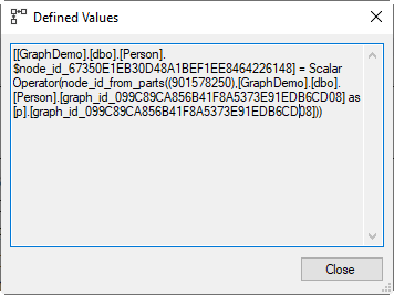Following the flow of the data, we first look at the Defined Values property for the right-most Compute Scalar operator. You can see it in the screenshot on the right.

As always with these kinds of expressions in execution plans, it is very hard to read due to the extra naming elements (database and schema), and all the often needless parentheses and brackets. When I remove those, as well as the hex strings for the generated columns names and the duplication caused by the table alias, what remains is effectively this definition:

Person.$node_id = Scalar Operator (node_id_from_parts (901578250, p.graph_id))

This does indeed confirm that the $node_id column is computed, rather than returned from the stored data by the Clustered Index Scan. Which definitively proves that sys.columns was lying to me; this column is most definitely a computed column. And we now also see how it is computed, using an internal scalar function called node_id_from_parts. This function takes two parameters, an object_id and a graph_id. The first parameter is 901578250, but it will be a different value on your system. This is, not coincidentally, the OBJECT_ID of the dbo.Person table. The second parameter is the value from the hidden internal graph_id column.

The functionality of the node_id_from_parts function is exactly as its name implies: it builds a node_id value (the JSON string that you see in the $node_id column of the output) from the input parameters. The object_id is used to determine the schema- and table-name that are included in the JSON. The graph_id is then used as the value for the “id” property. The JSON fragment has one more property, called “type”, and that is always set to “node” by node_id_from_parts.

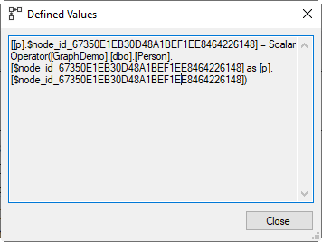The other Compute Scalar then has this Defined Values property (see screenshot on the right):

After applying the same simplification as for the previous expression, this essentially boils down to:

p.$node_id = Scalar Operator(p.$node_id)

Effectively, this does nothing. I assume that the reason for this extra Compute Scalar is simply an artefact of some internals of the compilation process. Normally, I would expect such a useless operator to be removed at the end of the compilation. But in this case, there is no need for such a cleanup. Both Compute Scalar operators in this case use deferred evaluation. Which in this specific case means that this superfluous Compute Scalar adds literally nothing to the execution effort. So in this case, even the little amount of work needed at the end of the compilation to identify and remove this useless Compute Scalar would be a waste of resources.

So the bottom line of reading this execution plan, is that the Clustered Index Scan reads the two columns we explicitly created (ID and name), plus the hidden internal column graph_id. The Compute Scalar then uses the latter and the object_id of the Person table, to construct the $node_id column that is returned to the client. This definitively proves that the $node_id column is, in reality, not stored on disk, but implemented as a computed column. And the is_computed column in sys.columns is a dirty little liar.

So now we know that a node table stores not only the columns that we supply when creating the table, but also two additional, generated columns. The $node_id column is not really secret; just running a SELECT * query on any node table will reveal the existence of this column, and show its contents. The graph_id column is hidden only slightly better. It cannot be queried, but its presence can be seen from sys.columns, or even by expanding the columns node in Object Explorer. Despite the lies that sys.columns tries to tell us, we know that the JSON text in $node_id is not actually stored; this is a computed column, based on the object_id of the node table, plus the value in the hidden graph_id column.

To the edge!

Now that we know the actual structure of node tables, let’s shift our attention to the other ingredient of graph databases: edge tables. They are designed to store relationships between nodes in a very efficient and flexible way. In a traditional relational database. If you want to store what restaurants people like, what cities they like, and also what other people they like, you’d have to use three separate foreign key relationships. And in this case they’d all be many-to-many relationships, so they’d have to be implemented as three separate tables. A graph database can use just a single “likes” table to store all these.

Let’s look at the details of an edge table to understand how exactly these various relationships are stored in that single table.

SELECT *
FROM   dbo.likes AS l;

We once more see that SQL Server has created additional columns. The CREATE TABLE statement for dbo.likes listed only a single column, rating. And yet, the results of the above statement show a total of four columns:

The three additional columns that SQL Server has generated are called $edge_id, $from_id, and $to_id. (Just as with $node_id in the node table, there is no need to type in the long hex string that SQL Server has added; SQL Server can handle this internally). And when you look carefully at the data above, and compare that to the data that was inserted in the dbo.likes table, you’ll notice that $edge_id is used as a way to uniquely identify each edge in the database, just as $node_id does for nodes. And you’ll also quickly realize that both $from_id and $to_id are references to the $node_id coluns in the various node tables.

Because the name of the node table is part of this data, multiple different “likes” relationships can now be stored in this same table. The sample data happens to only have “person likes restaurant” data, but if you add a row to represent that, for instance, Mary likes Redmond, or that Jacob likes John, then you will see that the $to_id column is now populated with data where the table property in the JSON is different for some rows.

Let’s now also check whether SQL Server has additional, hidden columns for edge tables, just as it does for node tables.

SELECT column_id,
       name,
       is_computed,
       is_hidden,
       graph_type,
       graph_type_desc
FROM   sys.columns
WHERE  object_id = OBJECT_ID ('dbo.likes');

Here are the results on my system:

As you see, there are even a whopping five (!!) extra, hidden columns generated for an edge table: graph_id, from_obj_id, from_id, to_obj_id, and to_id.. Based on the name, you might already have a suspicion what they are used for. But why go by suspicion when we can find out for sure through no more effort than the analysis of the execution plan for one simple query?

SELECT *
FROM   dbo.likes AS l;

Here is the execution plan for the above query:

This execution plan looks remarkably similar to the execution plan we previously saw when we queried a node table. The only clearly visible difference is that this time, we get a Table Scan, rather than a Clustered Index Scan. That is because we declared a primary key (which by default creates a clustered index) when creating the Person table, and did not do so when we created the likes table.

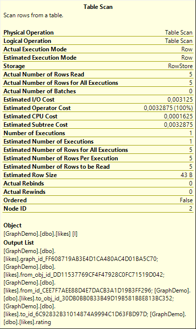The Output List property of the Table Scan (as shown in the screenshot on the right) gives us a first clue that the JSON columns, all three of them, are in fact not stored in the table, but implemented as computed columns. The data returned are effectively all other columns: the graph_id, the from_obj_id and from_id, the to_obj_id and to_id, and of course our own column, rating.

For final confirmation, we can also inspect the two Compute Scalar operators. The left-most one is superfluous, just like the one we saw before when looking at the node table. The Compute Scalar on the right computes, in this case, not one but three columns. Here are the three Defined Values expressions, in heavily simplified form:

likes.$edge_id = Scalar Operator (edge_id_from_parts (981578535, likes.graph_id));
likes.$from_id = Scalar Operator (node_id_from_parts (likes.from_obj_id, likes.from_id));
likes.$to_id = Scalar Operator (node_id_from_parts (likes.to_obj_id, likes.to_id))

The computation of $edge_id is very similar to what we previously saw for the $node_id in the node table, except that a different internal scalar function is used: edge_id_from_parts. This function does the same as node_id_from_parts, but now for an entry in an edge table, rather than in a node table. The first parameter (object_id) is once more hard-coded, and represents of course the object_id of the likes table; the second parameter is the graph_id. So this is, apart from the function name, effectively the same logic we already saw when we inspected the nodes table.

Both $from_id and $to_id are computed using the internal scalar function node_id_from_parts that we already saw before. In this case, object_id is not hardcoded, but taken from from_obj_id or from_to_id; the from_id or to_id columns are used as the graph_id parameter. Together, these two columns are a reference to one entry (graph_id) in a node table (object_id).

Conclusion

When you create graph tables, SQL Server will create some extra columns for you, under the cover. Some of these can be accessed, others are hidden. All of these columns have a name that ends in a long hexadecimal string, but those that can be accessed are also recognized by the short version of the name, without that hex string.

A node table has two of these generated columns. The inaccessible graph_id column holds a generated bigint value that is used to uniquely identify entries in that table; the $node_id column is a computed column, that holds a JSON string that combines “node”, schema- and tablename of the node table, and the graph_id. This is a system-wide unique identifier for each node (though in a format that is more user-friendly than computer-friendly).

An edge table has a similar mechanism for uniquely identifying entries, once more with a hidden graph_id column for a unique number, and this time the human-readable JSON string is in the computed column $edge_id. There are also two other columns, $from_id and $to_id; the values in those columns are all equal to the $node_id of an existing node, so they can be used to store the begin- and end-point of each edge. However, these two JSON columns are also computed, based on four hidden columns: from_obj_id, from_id, to_obj_id, and to_id.

All this might appear to be only moderately interesting, but it will become more important in my next blog posts about graph tables. After all, SQL Server does not generate those columns just for fun. They are in fact heavily used in the execution plans for graph-based queries, and that is why it is important to know that these columns exist, and understand what they are used for.

As always, please do let me know if there is any execution plan related topic you want to see explained in a future plansplaining post and I’ll add it to my list!