Welcome to part twenty-two of the plansplaining series, where we will continue our look at execution plans for graph queries. We started this series by investigating the hidden columns in the internal structure of graph tables. In the second part, we looked at how those hidden columns are used in the execution plan for a relatively basic graph query. Time to up our game and tackle the SHORTEST_PATH function, introduced in SQL Server 2019, that can be used to make SQL Server search a graph iteratively or recursively to find the shortest possible path from one node to another.

Sample data

I will continue to use sample tables and data from Microsoft’s documentation. You can find the script to create and populate the tables here, or in my first post on SQL Graph.

Please note that I used the sample exactly as provided. This sample does not follow Microsoft’s own indexing best practices. For edge tables, especially for those that are used in SHORTEST_PATH expressions, Microsoft recommends creating indexes ($from_id, $to_id) and on ($to_id, $from_id). But those are not created in the published sample tables, so I decided not to add them. I plan to look at performance of graph objects and graph queries later, and at that time I will of course investigate the effect of this best practice recommendation.

SHORTEST_PATH

Let’s first look at what SHORTEST_PATH actually does, and how to use it in a query. Let’s say that we need to know everyone who are friends of Jacob or Julie. That would be done with a normal graph query, just like those we used in the previous post:

SELECT p1.name AS PersonName,
       p2.name AS FriendName
FROM   dbo.Person   AS p1,
       dbo.friendOf AS fo,
       dbo.Person   AS p2
WHERE  MATCH(p1-(fo)->p2)
AND    p1.name IN ('Jacob', 'Julie');

The only difference with the sample queries from the previous episode is that I have now used table aliases. I could have done that in the last episode as well, but I chose not to, because I felt the queries would be easier to understand when using the full names of the node and edge tables. However, we now use two copies of the same table, so in this case we must provide an alias for at least one of them.

In the results you will see that Marie is a friend of Jacob, and Jacob is a friend of Julie. However, Julie is not a friend of Jacob. SQL Graph only uses “directed graphs”, which means that data in edge tables cannot be read in both directions. If your real-world problem needs an undirected graph, then you will have to store each edge twice, once for each direction.
(And as a side node, just from the data in the Person and friendOf tables in the sample data alone, any soap series would be able to fill at least three seasons!)

I am not going to show the execution plan for this query. It is very similar to those we have already seen. The only tricky part is to make sure to understand, when an operator accesses the Person table or an index on it, whether it is for the first or the second copy of that table (p1 or p2).

But what if we also want to see the friends of the friends of Jacob and Julie. And then their friends as well? That’s where the SHORTEST_PATH function comes in. This function finds all possible paths from one node to another across specified edges, and then return the shortest path (or, if there are multiple paths of equal length, returns one of them). This is the logical description, the actual implementation is optimized, as we’ll see in the rest of this post.

Here is how you can rewrite the previous query to use SHORTEST_PATH to find friends, friends of friends, and friends of friends of friends, of Jacob or Julie:

SELECT p1.name                                             AS PersonName,
       COUNT(fo.$edge_id)        WITHIN GROUP (GRAPH PATH) AS Distance,
       STRING_AGG(p2.name, '->') WITHIN GROUP (GRAPH PATH) AS FriendshipPath,
       LAST_VALUE(p2.name)       WITHIN GROUP (GRAPH PATH) AS FriendName
FROM   dbo.Person            AS p1,
       dbo.friendOf FOR PATH AS fo,
       dbo.Person   FOR PATH AS p2
WHERE  MATCH(SHORTEST_PATH(p1(-(fo)->p2){1,3}))
AND    p1.name IN ('Jacob', 'Julie');

The SHORTEST_PATH function can be found within the MATCH expression. Its argument looks similar to the argument we saw used directly in MATCH in the previous episode, an almost visual representation of the relationship between, in this case, two persons where one must be a friend of the other. However, there is a subtle change you might overlook: from p1-(fo)->p2 to p1-((fo)->p2). The extra parentheses around “friend of person two” indicate that this part may be iterated recursively. And then, just after that pattern, we see {1,3}, which means that we want at most three recursions (so no friends of friends of friends of friends). You can increase or decrease the maximum recursions by changing the second number, or you can allow infinite recursion by replacing the {1,n} pattern by a simple + sign.

The two tables that appear in the recursive part now also have an additional “FOR PATH” specification in the FROM clause. This is required for all edge and node tables that are used in any SHORTEST_PATH function, and it is not allowed for any other tables. This indicates that the query does not return a single friendOf row and a single Person (p2) row for each row in Person (p1), but that an ordered collection of all edges and nodes along the path is returned for each Person (p1).

But the SELECT list cannot project data from those ordered lists directly. To work around that, we must include all columns from friendOf and from the second instance of Person within aggregate functions. The aggregation will be applied to the ordered collection, to then return a single scalar value that can be returned to the client.

Note that the sample above uses COUNT(fo.$edge_id). You might have expected to see COUNT(*) here, but that is not allowed in SHORTEST_PATH queries. This is because the edges in the ordered list that COUNT(…) operates need not necessarily be of the same type. In the sample query, they can only be “friendsOf” edges. But in a more complex example, the shortest path could go across different types of edges. For a path that traverses four “friendsOf” edges and two “livesIn” edges, should the COUNT function return two (for livesIn), four (for friendsOf), or six (for the grand total)? I personally would assume * to mean any, so I would expect six. But it seems that Microsoft has chosen to remove this possible source of confusion, by insisting that you always specify the column to be counted, which obviously implies which edges are counted. (To get the grand total of livesIn and friendOf edges, you’d have to use two COUNT expressions and add them together).

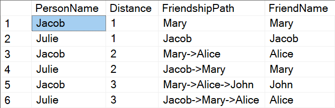
With all these changes, the query works, and returns the expected results:

Execution plan

But who cares about the results of a query, right? We want to see execution plans, those are much more exciting!

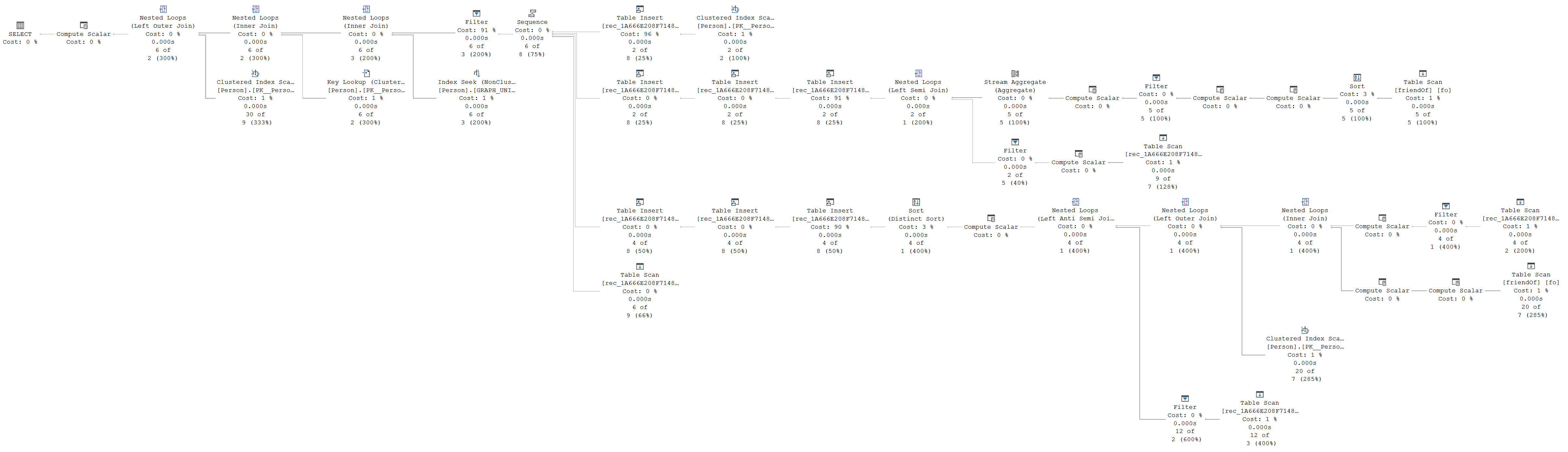
Uh, really? Exciting? Surely you mean overwhelming and scary, right? (BTW, you can click on the picture to see a full screen version, which might be easier to read. Or you can just execute the query and get the same execution plan in your SSMS or ADS window)

Well, no. Admittedly, it’s a very daunting execution plan. Analysing it won’t be a walk in the park. But it’s too hot for a walk in the park anyway, so let’s just dive right in.

When execution starts, the SELECT “operator” calls its child, Compute Scalar – except that this Compute Scalar uses deferred evaluation, so it doesn’t actually execute and in reality, SELECT directly calls the left-most Nested Loops. From there on, each operator immediately calls its child, and soon control is passed to the Sequence operator.

Sequence

The task of a Sequence operator is simply to execute each of its inputs, in sequence, while discarding all results that are returned (if any). Only the results from the very last input will be returned to its parent.

So in this case, because this Sequence operator has four inputs, the first three are only for preparation work. Only the last (fourth) input to Sequence produces relevant results for the rest of the query, that Sequence will pass on to its parent operator.

Since the four inputs execute in order, let’s inspect them in order.

First input

The first input to the Sequence operator is really simple:

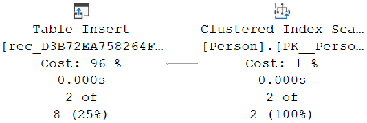
The Object property of the Clustered Index Scan revels that it reads data from the clustered index on the Person table, aliased as p1. There is also a Predicate property, to filter data and only return rows where p1.name is equal to ‘Jacob’ or ‘Julie’. The Output List property shows that just one column is returned: the graph_id column (for easier reading, I will consequently omit the semi-random hex strings in all columns names).

Both the alias used in the Object property (and a few other places) as well as the filter on the name column in the Predicate makes it very clear that this operator reads the data from the Person table aliased as p1. Basically, the start of our search for the shortest friendship paths to the other persons (p2).

As expected, the run-time statistics in the execution plan show that this operator reads all five rows in the Person table, to return just two of them. Julie and Jacob.

Those two rows are then passed into a Table Insert operator. This operator inserts data into a heap table. The Object property of the Table Insert reveals that the target of this insert is, in this case, a table in tempdb, named rec_xx­_source (where xx is yet another long hexadecimal string that is different each time the execution plan gets recompiled).

Do note that the optimizer can choose between two strategies here. In this case, the rec_xx_source table was populated from the persons named Julie and Jacob, basically the starting point or left-hand side of the paths we’re going to search for. The optimizer could also have chosen to put the ending point, or right-hand side, in rec_xx­_source (and then make appropriate modifications to the other branches). In this case, that would have been the entire Person table, because there is no filter on the p2 table. If you modify the query to add for instance a filter on FriendName = ‘Mary’, then the optimizer might make a cost-based decision to do this reverse search instead.

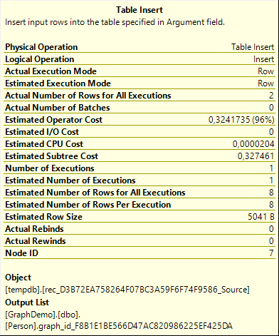
To get more information about this table, we need to look at the full properties list, instead of at the popup.  Here, the Object property can be expanded, to get some additional details.

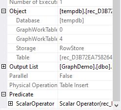As you can see in the screenshot on the left, the Storage subproperty indicates that the target table is a good old regular rowstore table. But more interesting are two other properties: GraphWorkTableIdentifier and GraphWorkTableType, set to 0 and 4 respectively. I’ll get back to the exact meaning of these properties later. For now, it suffices to say that these identify the target table as a special internal worktable, that is automatically created for the duration of this query and then removed again.

Since this is an automatically generated internal table, we do not know its structure. And yet, we can get a fair idea of that structure, by looking at the Predicate property of the Table Insert. The screenshot above shows it partially expanded. You can keep expanding it if you want (it’s quite a few nesting levels deep), or you can use copy/paste to get the text of the Predicate in an editor, where you can then edit it manually to make it more readable. Note that the name of the target table is truncated in this property.

After editing for readability, the property looks like this: “Scalar Operator (rec_xx_source.[graph_id] = p1.graph_id)”. In other words, the table rec_xx_source has just one column, named graph_id, and it gets populated with the graph_id of the rows from Person (p1) that meet the WHERE clause.

Second input

The second input to the Sequence operator is a lot more complex. Here is a screenshot of just that part of the execution plan:

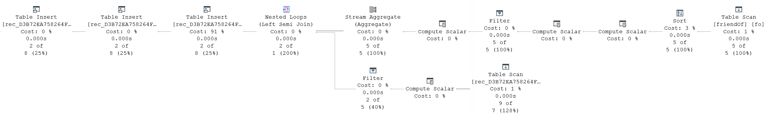
(Click on the image to see a larger version)

The sheer number of operators makes this look complex, but if you just check each operator one by one, you’ll see that nothing really special is happening here. However, to keep the size of this blog below that of Tolstoy’s War and Peace, I’ll switch to a more global description of what’s going on in this branch of the execution plan.

Top input to Nested Loops

Let’s start with the top input to the Nested Loops operator. Data is read from the friendOf edge table by a Table Scan operator, that reads all rows without filter, and returns all five columns: graph_id, from_obj_id, from_id, to_obj_id, and to_id. Those rows are then sorted by (to_id, from_id). The left-most Compute Scalar then uses the edge_id_from_parts function to compute the $edge_id column, based on the graph_id and the (hardcoded) object_id of the friendOf table. The next Compute Scalar sets this value equal to itself. As explained in earlier episodes of this series, the optimizer often doesn’t remove useless Compute Scalar operators, especially when they use deferred evaluation. Note that the only reason why SQL Server computes the $edge_id here is because it is used in the COUNT expression in the query. This could be avoided if COUNT(*) was supported for SHORTEST_PATH queries, but that is unfortunately not the case. In this case, I could have saved a bit of performance by using COUNT(p2.name), because that saves a bit of computation and also a bit of space in the internal tables that we’ll see shortly. But the results could also, under some circumstances, be different.

After having added the $edge_id column, a Filter operator reduces the amount of rows by applying a Predicate on from_obj_id and to_obj_id. Both must be equal to the object_id of dbo.Person (which is stored as a hardcoded value in the execution plan). With our sample data, this does nothing. But if you have played with the data and added additional edges to represent that cities like restaurants, or that persons like cities (which of course don’t all make sense in the real world, but they are permitted in this database), then those edges will now be removed from the data. Only the “person likes person” edges now remain.

Yet another Compute Scalar adds four extra columns to the data, Expr1002, Expr1003, Expr1004, and Expr1005. They are set to 1, 0, 0, and NULL respectively. The reason for this will become clear later. Finally, a Stream Aggregate operator aggregates the data by (to_id, from_id). This is required because the tables in our database allow us to store “Alice likes John” two, three, or even a hundred times. Those duplicates do not affect the shortest path, so they are removed here. The Defined Values property of the Stream Aggregate uses the ANY aggregate function (not allowed in T-SQL, but available internally in execution plans) to just pick one of the $edge_id values to be retained from those duplicated rows. (It uses ANY on all other output columns as well, but they all have the same value anyway, so here it does not really matter).

The Sort operator is only included in this branch of the execution plan because Stream Aggregate expects its input data to be ordered. In this case, using Sort + Stream Aggregate was, apparently estimated to be cheaper than using Hash Match (Aggregate).

The total effect of this branch is to find friendOf edges that connect two persons, remove duplicates from this collection (if any), and then return a total of nine columns: $edge_id, from_id, from_obj_id, to_id, to_obj_id, and the four new columns Expr1002, Expr1003, Expr1004, and Expr1005, that are set to 1, 0, 0, and NULL respectively.

(Note that just in this branch alone, there are some huge missed optimization opportunities. Why is the Filter not pushed past the Sort operator, so that only the reduced set of data is sorted? And once that push is made, why not push it even deeper, inside the Table Scan operator, so that the filtering can be directly done by the storage engine? Also, why not wait with adding the four Exprnnnn columns until after  the aggregation that removes duplicates?)

Nested Loops and its bottom input

The bottom input from the Nested Loops reads data from a Table Scan on the table that was populated in the first branch, rec_xx_source. We already know that this internal table has just a single column, graph_id, so it’s no surprise that the Defined Values property shows that only this column is returned. A Compute Scalar operator then effectively just renames this column, by setting Person.graph_id equal to rec_xx_Source.graph_id. And a Filter operator then compares this newly formed column Person.graph_id to friendOf.from_id (which is pushed into this branch by the Outer References property of the Nested Loops), and allows only rows where this is True to pass.

The Nested Loops itself has its Logical Operation set to Left Semi Join, which means that it does not actually add data from the bottom input to the top input. It only filters the data from the top input. Basically, this does an EXISTS.

All combined, the total effect of the Nested Loops with its bottom input is to take the top input (described above), and then apply a filter that only allows rows where the “from” part of the edge appears in the rec_xx_source table. Or in other words, we now have all the edges that represent “(Julie or Jacob) likes (some person)”, with duplicates removed. And we still pass on the same nine columns that Stream Aggregate returned to Nested Loops.

Table Inserts

The data that Nested Loops returns then passes through three Table Insert operators. At first glance, you might believe that all three insert data into the same table, because all these operators target an object starting with rec_ and then every time the same hexadecimal code. However, if you look at the full table name, you will see that they are not the same. Going from left to right, these three operators insert data into rec_xx_Results, rec_xx, and rec_xx_Total.

All of these three internal tables are rowstores, all of them with GraphWorkTableIdentifier equal to 0, but their GraphWorkTableType properties are different: 3 for rec_xx_Results, 0 for rec_xx, and 2 for rec_xx_Total.

Checking the Predicate property, I see that the data inserted into rec_xx_Results and rec_xx is exactly the same: l_obj_id = fo.from_obj_id, l_id = fo.from_id, r_obj_id = fo.to_obj_id, r_id = fo.to_id, rec_depth = Expr1002, col_1 = fo.[$edge_id], cnt_1 = Expr1003, cnt_2_y = Expr1004, and agg_1 = Expr1005. For the insert into rec_xx_Total, the third and fourth columns are named to_obj_id and to_id rather than r_obj_id and r_id; and the fifth column is not named rec_depth, but some guid, that changes whenever the plan is recompiled.

Based on the names of these columns, we can guess what their function is. I assume that l_obj_id and l_id stand for “left object id” and “left id”, whereas r_obj_id and r_id represent the right object id and id. Basically the same as the from and to object_id and id that are stored in the edge table, except now phrased in terms of left and right rather than from and to. The col_1 column holds the $edge_id column that we need for the COUNT function. rec_depth is the recursion depth (remember, SHORTEST_PATH does a recursive search for paths between nodes); we’re not at the recursive part yet, so it makes sense that this value is always 1. The cnt_1 and cnt_2 columns probably store some counters, both currently still at 0, and the agg_1 column is used for some aggregation; this column is initialized at NULL. What exactly is counted and aggregated in these columns will become clear as we look at the third input to the Sequence operator.

(Note that the columns col_1, cnt_1, cnt_2, and agg_1 are not actually called that, they are named col_xx, cnt_xx, and agg_xx, where each xx is once more some unique hex string. But using _1 and _2 makes it all easier to read and comprehend  And just in case you are wondering – yes, when I changed the SELECT list to return additional columns, extra col_xx, cnt_xx and agg_xx columns were added to these tables).

Bringing it all together

So let’s summarize the total effect of this second input to the Sequence operator. We find all the “friendOf” relations that originate from the rows that were added to rec_xx_source in the first branch and go to another person. In other words, we find all Julie’s and Jacob’s friendships. These are then stored in three different tables, that therefore are at this time identical. They contain those selected edges, where the naming has been changed from “from and to” to “l and r” (for left and right), and with some columns to track recursion depth and some counters and aggregations, initialized to 1, 0, and NULL initially.

Technically speaking, there is no need to do this in two steps. The bottom input of the Nested Loops could have searched directly in the Person (p1) table, with the filter on p1.name. That would in this case probably be slightly faster, and even more so when I create an index on the name column, with $node_id included. But even though that index will then be used in the first input to Sequence, the two inputs will never be collapsed. I assume that this Sequence with its four inputs is a standard pattern for SHORTEST_PATH queries, and that the optimizer is unable to work at the level where that first input is moved to the bottom input of the Nested Loops in the second input. (Also, don’t forget that in realistic queries, the first input is likely more complex than a simple Table Scan or Index Seek, and you probably don’t want those more complex inputs on the lower input of a Nested Loops!)

Anyway, at this point we now have four internal tables. Rec_xx_Source stores data from Person for Julie and Jacob; rec_xx_Results, rec_xx, and rec_xx_Total all store data from friendOf for only Julie’s and Jacob’s friends, with some extra counters, and equal in all three tables.

Third input

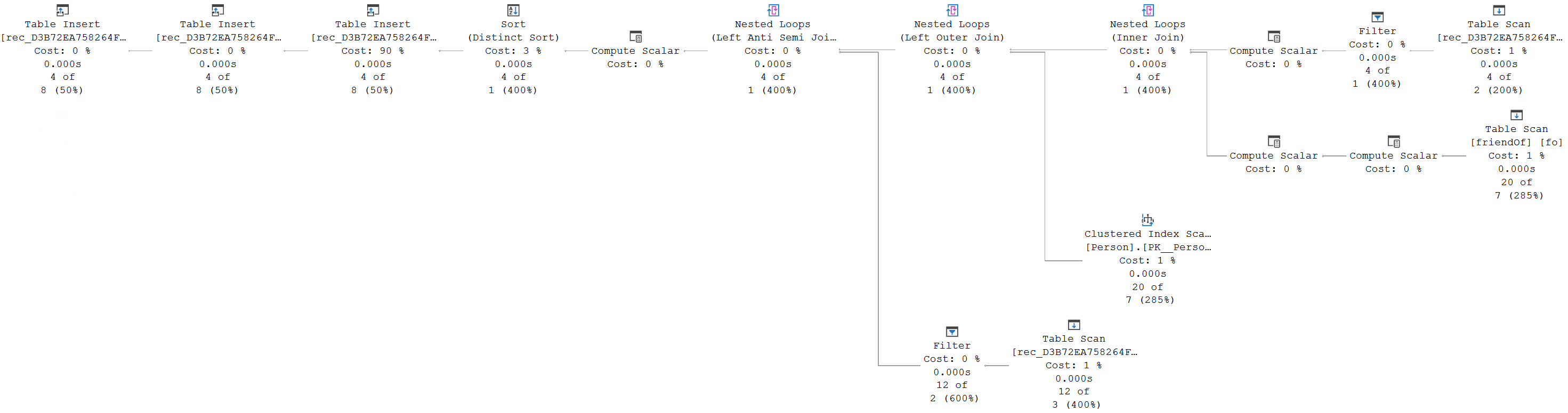
The third input has even more operators than the second input. But, I promise, it is not really any more complicated. Just a lot of operators, so you’ll once more have to click the screenshot below to expand it to full size:

Recursion

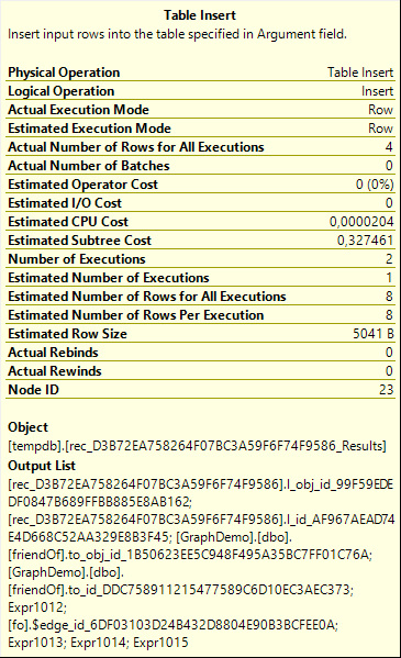Before I even start to look at the (rather complicated) branch of operators that is the third input to the Sequence operator, I want to point out a detail that is in this case very important. You can see it when you look at, for instance, the first Table Insert operator on this branch. See the screenshot on the right.

Pay special attention to the Number of Executions property. As you see, this operator executed twice. That is weird. I would normally expect the Number of Executions to always be 1, except for operators on the inner (lower) input of a Nested Loops operator. This Table Insert is not on the lower input of any Nested Loops. So why did it execute more than once?

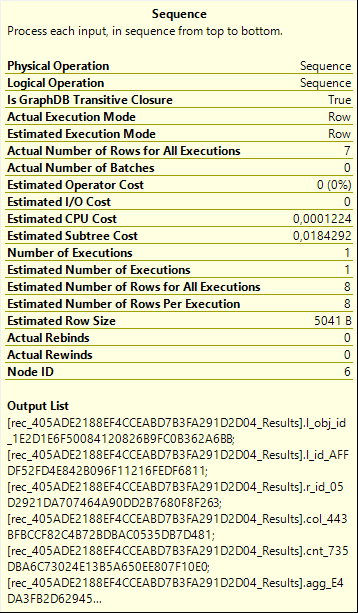The answer to that question can be found when we return to the Sequence operator. Let’s take a look at its properties. If you look, you’ll see something there that is not normally found in the properties of a Sequence: a property called Is GraphDB Transitive Closure, with a value of True.

Also, not visible in the properties popup, but present in the full properties window of this operator, is another graph related property, called GraphSequenceIdentifier. This property has the value 0 in our execution plan.

These two properties are used exclusively (as far as I know) for queries that use SHORTEST_PATH. The most important one is the one that we can see on the popup: Is GraphDB Transitive Closure. This property tells Sequence that it should modify its behaviour slightly. Instead of executing all inputs exactly once, from the first until the last, it has to execute its second-last input (so the third input in this case) multiple times, until a certain stop condition (that I’ll describe later) is reached.

This makes sense, when you think about it. SHORTEST_PATH is supposed to recursively look for paths. In this case up to three recursion levels deep, because we specified {1,3} in the query, but we can change that to {1,6} to allow more recursion, or to + to allow infinite recursion, and the shape of the execution plan does not change. By setting : Is GraphDB Transitive Closure to True, the Sequence operator gives us exactly that recursion, by repeatedly executing the second-last input until the stop condition becomes True.

Rightmost Inner Join

On the far right of this recursive third input to the Sequence, you find a Nested Loops that combines two inputs. Its top input reads from the table rec_xx, one of the three tables that was populated in the second input to Sequence with the friendships of Jacob and Julie. This is the starting point for the recursion. The Filter operator seems useless, it filters on the r_obj_id column to make sure we’re only working with friendships to a person, but since we already had that same check in the second branch, I do not see how this Filter would ever refuse a row. Perhaps there are some more advanced SHORTEST_PATH patterns that I have not tried yet where this Filter does serve an actual purpose.

The Compute Scalar to the right of this Filter is actually quite interesting, because it does some very relevant computations. After simplifying, the Defined Values property reads:

Expr1012 = rec_depth + 1; Expr1013 = CASE WHEN col_1 IS NULL THEN cnt_1 ELSE cnt_1 + 1 END

In other words, here is where the recursion depth is increased, in Expr1012. We also see, in Expr1013, one of the counter columns increased, but only if the column col_1 ($edge_id) is not null. That is the standard logic for the COUNT(fo.[$edge_id]) expression in the query. Even though the $edge_id of the friendOf edge can never be null, this pattern still includes this test. There is not enough performance to be gained by including extra optimizer logic for this.

The second input to the right-most Nested Loops on the third branch reads friendsOf. The two Compute Scalar repeat a pattern we’ve seen before to compute the $edge_id for the rows that were read from the graph_id and the object_id of the friendOf table. The Nested Loops itself than does an inner join, based on friendOf.from_id = rec_xx.r_id. Remember that r_id stands for the graph_id on the right side of the edge, also known as the to_id.

Effectively, this Nested Loops finds the friends of the friends that were found in the second branch.

Two more Nested Loops

The next Nested Loops (when following the data) is a Left Outer Join to the Person table. It tries to find a Person row with graph_id equal the r_id from rec_xx (so for the first iteration, this person would be a friend of Jacob or Julie, not the friend of a friend that was just added – this friend of a friend is currently stored in columns friendOf.*). When this person is found, their name is added to the returned columns.

Because the Logical Operation is a Left Outer Join, no rows are discarded when there is no matching rows in Person. In that case, the name column is simply set to NULL. This shows an interesting point. Graph tables allow us to create edges between nodes that don’t exist. Or to delete nodes while keeping the edges that were connected to them. In those cases, the edges can still be trailed to form a connection, even when the node itself no longer exists. If you want to see this in action, you can delete Alice from the Person table and then re-run the query. You’ll get the same results, but there will be no name in the FriendName column for two of the rows, and for one there will be only two names in the FriendshipPath, even though Distance indicates that the friends are three hops apart. All because Alice now still exists in the paths defined by the friendOf table, but no longer can be found in dbo.Person.

The left-most Nested Loops does a Left Anti Semi Join. This is roughly equivalent to doing WHERE NOT EXISTS. In other words, if a row from the top input has a match in the bottom input, then it is discarded.

The bottom input in this case searched in one of our internal tables: rec_xx_Total. This is where all edges travelled so far are stored. By looking in this table for the edge we are about to add to the internal table, we prevent endless loops. The sample data I used happens to not include any such loops, but it’s easy to add one. Just add a row in the friendOf table, as follows:

INSERT dbo.friendOf
VALUES ((SELECT $NODE_ID FROM Person WHERE ID = 2),
        (SELECT $NODE_ID FROM Person WHERE ID = 4))

Now we have rows for Jacob is a friend of Mary, and Mary is a friend of Jacob. Run the query, and you’ll see that this adds, for instance, a row for the friendship path from Jacob to Mary and then back to Jacob. It makes no sense to then further extend from here, because at that point we’ll always only find combinations of nodes where a shorter path without the loop from Jacob to Mary and then back to Jacob. And hence this anti semi join ensures that we don’t keep repeating the same pattern over and over. (And this is of course extra important when we change the recursion limit from 3 to endless, by replacing {1,3} in the query with a simple + sign – otherwise the recursion would literally be endless, and the query would never finish!)

Final logic

To the left of the three Nested Loops operators, we find another Compute Scalar. Here, a few more important computations are done. Here is the Defined Values property, once more heavily simplified for easier understanding:

Expr1014 = CASE WHEN p2.name IS NULL THEN cnt_2 ELSE cnt_2 + 1 END;
Expr1015 = CASE WHEN rec_xx.agg_1 IS NULL THEN p2.name
                WHEN p2.name IS NULL THEN rec_xx.agg_1
                ELSE CONCAT(rec_xx.agg_1,'->', p2.name
           END

In other words, Expr1014 is cnt_2, increased when the Person we joined to does have a non-null name. And Expr1015 is set to that name if it’s still NULL (which is the case for the first iteration of this branch), or otherwise the CONCAT function is used to add ‘->’ and the name to whatever was already there. Effectively, this ensures that Expr1015 (which will later be stored back in the agg_1 column in new to be added rows) keeps a sort of running total for what will eventually be the STRING_AGG expression from the query.

After that, a Sort operator with Logical Operation Distinct Sort is used to sort the data and then remove duplicates from the data, based on the columns (rec_xx.l_obj_id, rec_xx.l_id, and friendOf.to_id). You can see this in its Order By property. Remember, at this point the columns from rec_xx represent one of the friendships of Julie or Jacob, with l_obj_id and l_id representing Jacob or Julie, and r_obj_id and r_id representing the friend. The column friendOf.to_id then represents a friend of that friend. By searching for and removing duplicates based on only the l_obj_id, l_id, and to_id, we are skipping the middle man or woman. So the effect here is that if, for instance, Jacob is friend of John and Mary, and both John and Mary are a friend of Alice, then we would now have two distinct paths of the same length from Jacob to Alice. One through John, the other through Mary. SHORTEST_PATH should return only one of them in such cases, and that’s why there is a Distinct Sort here that looks at only Jacob and Alice, while ignoring the middle node.

Note that the Sort returns far more columns than are listed in the Order By. There is in this case no specification for how those columns are computed. When we previously used Stream Aggregate to get rid of duplicates, this was needed, because Stream Aggregate can do all sorts of aggregation. Sort (Distinct Sort) cannot do that. When it finds a duplicate, it simply discards one of the duplicated rows and retains the other.

More inserts!

Finally, we have the data ready to be inserted into, once more, three internal tables. Beware, even though this section looks very much like the corresponding section in Sequence’s second input, it is not the same.

The main difference is that we don’t insert into the same three tables. The leftmost Table Insert does still insert into rec_xx_Results. And the rightmost still inserts in rec_xx_Total. But the target of the middle Table Insert is changed, now we’re inserting in rec_xx_IterateNext, with GraphWorkTableType 1.

Another quite subtle but very important difference is that now the data inserted in the r_obj_id and r_id columns (or to_obj_id and to_id for rec_xx_Total) is still taken from the to_obj_id and to_id columns from friendOf, but l_obj_id and l_id are set equal to the l_obj_id and l_id from the rec_xx table that was the input for this branch. In other words, to either Julie or Jacob.

This means that the rows that are now added “connect” Jacob or Julie (in the “left” columns) to the friends of their friends (in the “right” columns), without still storing the friend in between – except that some computed data from that friend in between is now present in the cnt_n and agg_n columns.

Because these rows were added to rec_xx_Total and rec_xx_Results, both those tables now have rows for the friend of Jacob and Julie, plus rows for friends of those friends. However, rec_xx_IterateNext is a new table, where now only the friends of friends are stored.

Iterate

At this point, the third branch of Sequence is complete. However, because Sequence has its Is GraphDB Transitive Closure property set to True, it will now execute the same third branch again! This is where the recursion finally really kicks off.

Of course, if we at this point just repeat the third branch without doing anything else, then we would once more read Jacob’s and Julie’s friends and then find their friends’ friends. That’s not what we want, we already have that, and we need to take it to the next level.

What we do want, is to repeat this third branch, not using the data that was stored in rec_xx in the second branch, but using the data that the previous execution of the third branch stored in rec_xx_IterateNext. How this is done is not documented. I can think of multiple methods to achieve this. For instance, they could truncate rec_xx (because that data is no longer needed), then use ALTER TABLE rec_xx_IterateNext SWITCH TO rec_xx (obviously as an internal command, so probably a bit faster) to effectively swap the two tables, making rec_xx contain what was in rec_xx_IterateNext, while rec_xx_IterateNext is once more empty, ready for the next iteration.

Another alternative would be to drop table rec_xx, rename table rec_xx_IterateNext to rec_xx, and then allocate a new rec_xx_IterateNext, for the same end result with roughly the same amount of work. Or one could actually delete the data from rec_xx, then move all rows from rec_xx_IterateNext to rec_xx, but that would be very inefficient compared to the other options.

Regardless of implementation, once this is done, rec_xx contains the friends of Julie’s and Jacob’s friends, the logic of the third branch will find the friends of friends of friends, and then add them to rec_xx_IterateNext (as well as to the other tables). And then on the next repetition, these friends of friends of friends will be in rec_xx, and the friends of friends of friends of friends are found and added. And so on.

However, there are no properties in the Sequence operator that indicate which two tables it needs to swap and empty before each next iteration. It doesn’t need to. And, just to be clear, it also does not parse table names to look for rec_xx and rec_xx_IterateNext. Instead, it uses the GraphWorkTableTypes that we have seen before when looking at the Object properties of the Table Insert and Table Scan operator. Type 0 indicates the rec_xx table that holds the base rows for the current iteration, and type 1 is for the rec_xx_IterateNext, where the new rows for the next iteration are gathered.

When using more complex SHORTEST_PATH expressions, the execution plan can contain more than one Sequence operator with Is GraphDB Transitive Closure True. This is needed when there are multiple independent recursions going on. And this is where the GraphSequenceIdentifier of the Sequence, as well as the GraphWorkTableIdentifier of each of the work tables come in. In our example, they were all 0. When I ran a query with a more complex expression, I had two Sequence operators, and they had identifiers 0 and 1 respectively, and their work tables also had identifiers 0 and 1. So long story short, the Sequence knows which tables to switch and empty out, based on the identifier and the table type.

But how and when does the recursion stop? Well, if the query specifies that all shortest paths need to be found, regardless of recursion level (by using the + symbol rather than the {1,n} pattern), then the only reason to stop searching is when during an execution of the recursive third branch, no rows are added to rec_xx_IterateNext. This is easy to test for the Sequence operator. If an iteration produced any new rows, then they are inserted into the three tables, but each Table Insert operator also returns those rows to their parent So Sequence can check whether it received data from its child (the leftmost Table Insert of the recursive input), and if it did, then another iteration is useful. When no data is returned, then clearly no new rows were returned, and any extra execution of the recursive branch would be a waste of time because it wouldn’t do anything anymore.

However, if a maximum recursion level is specified, such as in the demo query where I specified {1,3} to stop at three recursion levels, then that is an extra stop condition. While it would in theory be possible to first do the full recursion and then filter out unwanted rows based on the rec_depth column in the internal tables, that would be a huge waste of performance. And luckily, Microsoft was smarter than this. That’s why we have only two executions for the operators on this recursive third input to Sequence. The second input was effectively the first recursion, the two executions of the third input and the second and third recursions, and then, because we specified {1,3}, no extra execution of this branch is initiated.

How this is tested is, once more, unclear. I need to speculate. One theory that I had for a while, that operators in the third branch include a filter somewhere on the recursion depth, is by now disproven. We have seen all operators, and there is no such filter. Also, if that were the case, then there would still be one extra execution of this branch, albeit one that returns no rows. The Number of Executions of the operators on this branch indicates that this is not the case. When the maximum recursion is 3, as in the demo query, the operators on the recursive branch have just two executions. (Remember, the second branch is effectively the first recursion level).

So instead, it is the Sequence operator itself that does this check. Once more, this can be done in multiple ways. It can check the recursion depth that the leftmost Table Insert returns (in column Expr1012, in this case – note that it will not always use the number 1012, but it will always be the fifth column returned). Once that is equal to the maximum recursion level, the recursive branch should not be restarted again. However, a probably even simpler solution is to have the Sequence simply use an internal counter in its working memory, that it increases whenever it (re)starts the recursive branch. When that counter ticks over from 2 to 3, two executions have been done, which means three recursion levels. That is the maximum, so the recursion is stopped.

Fourth input

Finally, we get to the fourth input to the Sequence. Finally a simple one again!

It’s a simple Table Scan, using rec_xx_Results as the input. There is no Predicate property, so all rows are returned. And its Output List property specifies that all nine columns are returned: l_obj_id, l_id, r_obj_id, r_id, rec_depth, col_1, cnt_1, cnt_2, and agg_1.

An interesting observation is that in this execution plan, there is actually (apart from the column names) zero difference between rec_xx_Results and rec_xx_Total. They seem to be redundant. However, I assume that there are scenarios that I have not yet seen where there actually needs to be a difference between the total collection of edges traversed (for the purpose of preventing endless loops), and the results collection of edges that need to be returned as the final results.

Because this is the final input to Sequence, these rows are then also returned to its parent.

Rest of the plan

The rest of the plan still does a lot of work, but nothing in this section is really interesting.

Following the data, we first see a Filter that, once more, checks that the left object_id refers to the Person table. Knowing how the data is generated, I see no way that this would ever not be the case, so either this is a case of lacking optimization, or there are more complex cases where this filter would actually be needed.

We then see two Nested Loops operators that join the data we have (which, if you recall correctly, are all references to start- and end-points of a path through nodes) to the Person (p1) table, via first an Index Seek and then a Key Lookup, to get additional data. In the Key Lookup, we also see a repetition of the filter on the p1.name column, to return only Jacob and Julie. I once more fail to see any reason for this, because we already ensured this in the first input to Sequence. But, again, this apparent redundancy might become relevant in more complex queries.

Then we have one more Nested Loops, to the Person (p2) table. This join uses the r_id column from rec_xx_Results to get the correct value for the LAST_VALUE expression in the SELECT list. This works because r_id (and r_obj_id, but we know already that this is the object_id of dbo.Person) is the last node in the path represented by each row processed.

Finally, the last Compute Scalar is needed to ensure that col_1 and agg_1 are updated to reflect the correct COUNT(fo.[$edge_id]) and STRING_AGG results. If you read carefully, you will have noticed that in the recursive input to Sequence, we constantly added the previous value to the aggregations, while adding a new edge to the path. So those aggregations were lagging the whole time; the last node was not added. That’s why the count is increased one more time here, and one more name gets added to the FriendshipPath.

Could this have been done in a simpler way? I think: yes. Why not set the counter to 1 and the string aggregation to the name in the second branch? And then, in the recursive third branch, increase the counter and add ‘->’ plus the name for the endpoint of the edge that is added? That would at least allow the removal of this last Compute Scalar. But I believe it would also (slightly) reduce the complexity of the Compute Scalar expressions in the recursive third input to the Sequence.

Summary

An execution plan for a query with a basic SHORTEST_PATH expression consists of two parts. The Sequence operator, with its four inputs, seems to be a standard construction. That’s why all the column names are pretty generic. This unfortunately results in some missed optimization opportunities. For example, in the sample query, the Clustered Index Scan in the first input to Sequence could have returned the name column, that then could have been stored in the work tables and returned to Sequence, and its parent operators. That would have eliminated the need for the Key Lookup in the left-hand side of the plan, which is only needed to retrieve that name. (And to filter on it, but that is also a redundant filter. Probably also because the SHORTEST_PATH section of the execution plan is a mostly standard structure that the optimizer only has a limited understanding of).

The first branch of the Sequence identifies the nodes that are the source of the recursive SHORTEST_PATH computation. The second branch then uses that to find the first set of edges; this can be seen as the first level of recursion. After that, the third branch executes repeatedly, to constantly repeat the same logic on the rows that were added in the previous recursion. The fourth branch then returns the final results from a work table that was filled in the second and third branches.

Complexity

The example used in this post uses the most basic form of the SHORTEST_PATH expression. The syntax allows us to make these expressions quite a bit more complex. And if we do, then the execution plans quickly get very much out of hand.

Here is an example where I combined two SHORTEST_PATH expressions in a single query. The query has no real use, it is quite nonsensical, but it is definitely possible to construct tables and data where a query such as this would actually be useful. Using the sample tables and data we have, I’ll make do with a nonsensical (but syntactically correct) example.

SELECT COUNT(fo.$edge_id)        WITHIN GROUP (GRAPH PATH) AS Distance,
       COUNT(fo.$from_id)        WITHIN GROUP (GRAPH PATH) AS Distance,
       STRING_AGG(p2.name, '->') WITHIN GROUP (GRAPH PATH) AS FriendshipPath,
       LAST_VALUE(p2.name)       WITHIN GROUP (GRAPH PATH) AS FriendName
FROM   dbo.Person            AS p1,
       dbo.friendOf FOR PATH AS fo,
       dbo.Person   FOR PATH AS p2,
       dbo.friendOf FOR PATH AS fq,
       dbo.Person   FOR PATH AS p3
WHERE  MATCH(SHORTEST_PATH(p1(-(fo)->p2){1,2})
         AND SHORTEST_PATH(LAST_NODE(p2)(-(fq)->p3){1,2}))
AND    p1.name IN ('Jacob', 'Julie');

To save some space (and to save myself a lot of time cutting and pasting plan fragments together to make it seem I captured it all in a single screenshot), I have this time decided to zoom out a bit in SSMS, and make a screenshot that shows most but not all of this scaled down execution plan:

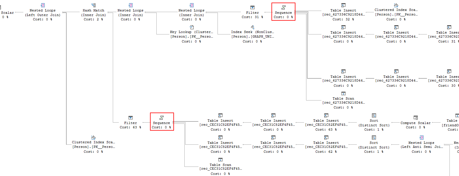
This execution plan contains two Sequence operators, marked in the screenshot above. Both have there is GraphDB Transitive Closure property set to True. And they have mostly the same inputs as the one in the execution plan we discussed above (with one notable exception, that I’ll cover in a bit).

This is where the GraphSequenceIdentifier and GraphWorkTableIdentifier properties gain relevance. They are 0 for the top-most Sequence, and for all work tables its child operators use. However, for the other Sequence, as well as the work tables used by it and its children, the identifier value is 1. Similarly, if you add even more complexity to the query, you might get even more Sequence operators to do transitive closure on part of the graph, each one with a higher value in the identifier properties.

You have of course noticed that the second Sequence in the screenshot above has only three inputs, instead of the four we have seen before. The reason for this is that this first branch is actually optional. If you want to see this in a much simpler query, then you can return to the query used at the start of this post and simply remove the filter on p1.name in the WHERE clause. Look at the execution plan, and you will see that the first input to Sequence is now gone, and the second input is a bit simpler.

The first branch is only needed when the SHORTEST_PATH algorithm needs to be executed on a selection of nodes from a node table. In that case, the first branch makes that selection and stores it in the rec_xx_Source table, which is then used as a filter in the second branch, the first step of the recursive iteration. However, when all nodes are selected, then SQL Server does not waste time to copy all nodes into a worktable and then filter edges based on a worktable that contains all nodes. Instead, it immediately starts with the first iteration, because we now know that all edges qualify anyway. So there now is no rec_xx_Source table, the first branch (that normally populates this table) is gone, and the second branch is slightly simpler, because it lacks the filter on the rec_xx_Source table.

But now the question is, why does the second pattern of a Sequence with its child trees use this unfiltered version? After all, the second SHORTEST_PATH does have a very clear filter, indicated by its starting point: LAST_NODE(p2). So we want to build upon the last person (or rather, the last friendship edge) from the first chain. Why is that filter not here?

I assume that this is a cost-based decision. SQL Server could have added the filter. But if you look at the properties in the execution plan, you’ll see that the cardinality estimator expects that 8 rows will be returned by Sequence, and then after two joins and a filter, this estimate is reduced to 1.78. (If you execute the query, you’ll that there are four in reality). If you want to use LAST_NODE(p2) as a starting point, then you’ll need to use a Nested Loops join, with an Outer References to push that starting point into its bottom input. That bottom input then executes an estimated 1.78 times, or in reality even 4 times.

The execution plan that is generated instead uses a Hash Match operator for the join. That means that the bottom input is guaranteed to be executed just a single time, regardless of the number of rows in the top input.

A single execution of the pattern of a Sequence and its child operators might be cheaper when all four branches are used to only work on the selected starting node, as compared to the version with three branches that finds all shortest paths. But on the bottom input of a Nested Loops, there is no single execution, there are multiple executions. In this case an estimated 1.78 executions, but that estimate might be wrong. The plan might already mathematically be more expensive purely based on cost times executions, but even when not, then it is still way more dangerous. If the estimate for the top input is wrong, execution time can really get out of hand, because the second SHORTEST_PATH Sequence is repeated as often as there are rows in that input.

Conclusion

In this exceedingly long blog post, we studied how SQL Server performs the “magic” behind the SHORTEST_PATH function. We saw that it optionally creates a starting set of nodes. It then first finds the edges for the first repetition of the recursive pattern, filtered by the results of the first step when applicable. And then it starts a recursive process, where each execution finds new edges to add, based on the edges that were added in the previous step, with some extra logic to prevent adding more than one path between the same nodes. All results found along the way are stored in a worktable, that is then finally used to return the final results.

All of this is orchestrated by a Sequence operator, that executes the three or four branches in turn. Some special extra logic in the Sequence operator ensures that it executes the second-last branch multiple times, until no more data is added, or until the maximum recursion level is reached. In between these executions, it empties and swaps worktables, so that the same operators on that recursive branch get new data every time, even though they read from the same table.

I saw a few things that made me raise my eyebrows, because they don’t seem optimal for performance. However, the amount of data used in this example was extremely small, which means that estimated plan costs were extremely low. At such low cost, the optimizer often tends to stop working early, because it makes no sense to spend hundreds of milliseconds optimizing an execution plan that finishes in less than ten milliseconds anyway. In the next part of this series, I will load the sample tables with lots of extra data to see whether these execution plans then change, and how performance of these graph queries is when tasked with serious data.

As always, please do let me know if there is any execution plan related topic you want to see explained in a future plansplaining post and I’ll add it to my to-do list!

P.S.: Thanks to Arvind Shyamsundar and his team for reviewing the first draft of this blog post, and providing invaluable feedback to improve it!