Welcome to part eleven of the plansplaining series. You will have noticed that this is no longer a monthly series. But when I was asked recently to provide some insight in how a MERGE statement is reflected in an execution plan, I realized that the plansplaining format works fine for this.

But first a word of warning. The MERGE statement, introduced in SQL Server 2008 as an easier alternative for “delete / update / insert” logic, turned out to have issues when it was released. And now, in 2020, many of those issues still exist. So I’ll just point you to Aaron Bertrand’s excellent overview, and leave you with the recommendation to be extremely wary before using MERGE in production code.

But here, we are not going to use MERGE in production. We are merely going to set up a simple test and look at how the elements in the execution plan cooperate to produce the expected results. This is interesting even if you never use MERGE, because many of the details explained below can also occur in other execution plans.

Sample scenario

For this post, I’ll create a relatively simple scenario, based on what is probably perceived as an ideal use case for a MERGE statement: synchronizing a table with product data based on a staging table that holds product data imported from an external source. New products must be added, modified data updated, and products no longer in the staging data are discontinued.

The tables

The scenario uses just two tables. One lists all products registered in our database. The second table is the staging table, that holds new product data from an external source. In this scenario the staging table always includes all current products, so if an existing product is missing from the staging table, we know it has been discontinued. The staging table includes the current price for each product. But to save bandwidth, the product name is only included if it was actually changed.

CREATE TABLE dbo.Products
    (ProductCode char(5)       NOT NULL PRIMARY KEY,
     ProductName varchar(40)   NOT NULL UNIQUE,
     Price       decimal(9, 2) NOT NULL,
     TotalSold   int           NOT NULL,
     Is_Deleted  char(1)       NOT NULL DEFAULT ('N'),
     CONSTRAINT CK_Is_Deleted CHECK (Is_Deleted IN ('Y', 'N')));

CREATE TABLE dbo.StagingProducts
    (ProductCode    char(5)       NOT NULL PRIMARY KEY,
     NewProductName varchar(40)   NULL,      -- NULL means no change
     Price          decimal(9, 2) NOT NULL); -- Always included

For simplicity sake, I have not included any sample data. Feel free to include some sample data of your own, if you prefer to see actual results from the query. My own experiments with small amounts of data did not affect the query plan shape. Loading huge amounts of data in the table might of course result in a different plan shape.

The MERGE statement

The query used to import the data from the StagingProducts table into the Products table uses this MERGE statement:

MERGE
INTO   dbo.Products        AS  p
USING  dbo.StagingProducts AS  sp
   ON  sp.ProductCode       =  p.ProductCode
  WHEN MATCHED
  THEN UPDATE
       SET     Price        =  sp.Price,
               ProductName  =  COALESCE(sp.NewProductName, p.ProductName)
  WHEN NOT MATCHED BY TARGET
  THEN INSERT (ProductCode,    ProductName,       Price,    TotalSold)
       VALUES (sp.ProductCode, sp.NewProductName, sp.Price, 0)
  WHEN NOT MATCHED BY SOURCE AND p.TotalSold = 0
  THEN DELETE
  WHEN NOT MATCHED BY SOURCE
  THEN UPDATE
       SET     Is_Deleted   = 'Y';

Most of this statement is pretty obvious if you know the syntax of the MERGE statement. If a product is in both tables, price get always updated, and name only when a new name is specified. A product that is only in the staging table is new, so it gets added. And if an existing product is not in the staging table, it is discontinued; in this case it is either physically deleted from the table, or retained but marked as deleted when any sales are registered on the product.

The execution plan

The execution plan for this query looks quite daunting, mostly because of the sheer number of operators used:

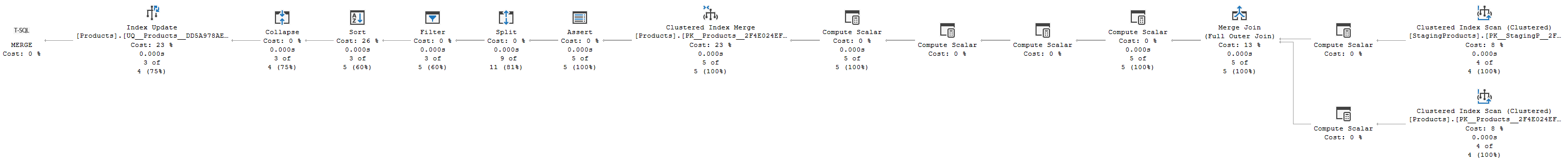
So let’s break this down section by section. In this case following the data (right to left) works better than following the control flow (left to right). So that’s what I’ll do.

Collecting the input data

Let’s start at the far right. This is where data from the two tables is read and combined.

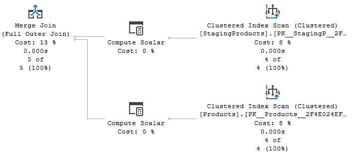
Two scan operators

Each of the two tables used in the query is read by a Clustered Index Scan operator. If you look at the properties you will see that no Predicate property is used, meaning that all rows from all tables are read into the execution plan. That is not the case for each execution plan with a MERGE statement. In this case, there are no other filters. The query wants to process all data, from both tables. For more complex queries, with filters on which rows to process and which to include, the optimizer will consider more advanced strategies using scans with a Predicate, or seeks, potentially combined with lookups. In this case, though, I want to focus on the actual MERGE processing, so the sample query simply reads all data.

Merge Join

The Merge Join operator on the left is pretty standard as well. The two indexes both produce data ordered by ProductCode, which is used as the join condition. So that means that a Merge Join is almost always more efficient than either a Nested Loops or a Hash Match. The logical operation of the Merge Join is a Full Outer Join. This is something that changes depending on the exact details of the MERGE statement. In this case, all three possible clauses (MATCHED, NOT MATCHED BY SOURCE, and NOT MATCHED BY TARGET) are included in the query, which means a full outer join is required. When less clauses are used, the execution plan will change this as needed to a left or right outer join, or (rarely) even to an inner join or a semi join.

Two Compute Scalars

But what about the two Compute Scalar operators in this section? What do they do? A Compute Scalar as the immediate parent of a scan operator is often caused by a computed column in the table definition, or to expressions on its columns in the query. But there are no computed columns in the tables used in the example. Nor are there any expressions that can be computed from merely the columns of one table.

The answer is of course in the properties. The screenshot shown here is from the Compute Scalar in the top branch. The Output List property shows that it returns the three columns it receives from the Clustered Index Scan on StagingProducts, plus one extra column called SrcPrb1001. The Defined Values property reveals that the computation for this column is extremely simple: it is merely set to the constant value 1.

In the bottom branch, you will see a very similar situation, where the Compute Scalar passes all columns read from the Products table and adds one new column, in this case called TrgPrb1003, and also set to the constant value 1.

Generated internal column names in execution plans always have a name that consists of a mnemonic code and a unique four digit number. The mnemonic code is often helpful to understand the purpose of the column. In this case, “SrcPrb” and “TrgPrb” are short for “source probe” and “target probe”. These columns are included to give other operators in the execution plan an easy way to verify whether a row they process include matched data from the source or target table, or no data. When I do this in my own queries I tend to check whether a column from one of the sources is NULL, but I do of course need to choose a column that cannot contain NULL values in the table. Rather than trying to find such a column, the optimizer simply uses this standard pattern to add a probe column to each row from each table.

Computing what to do

The next section of the execution plan is just four Compute Scalar operators in a line. The optimizer could probably have collapsed these into just one or two, but that would be an optimization with no measurable performance benefit, so it is just left as is. For easy reference in the text below, I have once more marked each Compute Scalar with its NodeID property in the screenshot below.

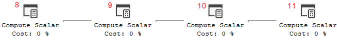
Compute Scalar #11

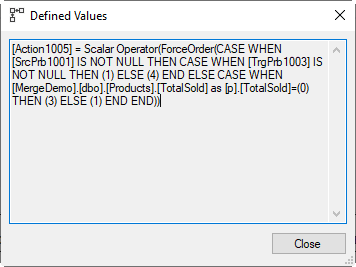We’re still following the data is it’s returned from one operator to another in response to their GetNext() calls, so let’s start at Compute Scalar #11. Its Defined Values property betrays that it computes just a single column, called Action1005. Here the name of the internal column is not exactly a mnemonic, it’s a full word. Columns named Actionnnnn are always “action columns”. You will always find them in plans for a MERGE statement, but I have seen action columns used in other plans as well.

Action columns are always used to encode a data modification action. Either one to be done, or one that has been done. The codes used are not documented, but from looking at execution plans such as this one and many others, I know at least these three possible values:

• 1: Update
• 3: Delete
• 4: Insert

The Defined Values property of a Compute Scalar is often hard to read. This one is actually relatively simple, we’ll see far worse below. But eve for this one, it can take some time to peel off the irrelevant parentheses and brackets, ignore functions such as ForceOrder that are there for technical reasons only, and understand the exact logic of the rest. I often use copy/paste into a query window and then use a combination of manual editing and SQLPrompt to reformat the Defined Values to an easier to parse format.

Action1005 = CASE WHEN SrcPrb1001 IS NOT NULL
                  THEN CASE WHEN TrgPrb1003 IS NOT NULL
                            THEN 1
                            ELSE 4
                       END
                  ELSE CASE WHEN p.TotalSold = 0
                            THEN 3
                            ELSE 1
                  END
            END;

In this format it is easier to follow the logic. Using nested CASE expressions, four different situations are distinguished. Going top to bottom, Action1005 is set to 1 (update) when both probe columns are not null. This corresponds to the WHEN MATCHED clause, which does indeed specify an update action. When the source probe is not null, but the target probe is null, meaning a row is present in the source table but not in the target table (“NOT MATCHED BY TARGET”), the action column is set to 4, insert. When the source probe is null, the target probe does not need to be checked. The optimizer knows that the Merge Join will only return rows that come from at least one table, so if no source data was used, then target probe has to be not null by definition, and this requires no check. However, the MERGE statement uses two “NOT MATCHED BY SOURCE” clauses. One with an additional test on p.TotalSold = 0, the other for the remaining cases. So that’s why here we see another nested CASE that uses this exact same condition to set the action column to either 3 (delete) or 1 (update).

So in short, the function of Compute Scalar #11 is to work out, for each row, whether the MERGE statement specifies that it results in an insert, update, or delete action.

(When you look at execution plans for other MERGE statements, where some rows may be not affected at all, you will see that those rows are typically filtered before the action column is determined. It might be possible that there are execution plans where an action column can result in a “no operation” value, but I have never seen such cases).

Compute Scalar #10

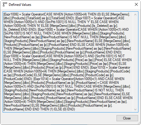The execution plan has now determined what needs to be done. The next step, Compute Scalar #10, is to work out the target values. And as you can see in the screenshot on the right, this is where the Defined Values property can get really messy.

This is in part because this operator computes not one but six new columns, which of course adds to the code in the Defined Values property. But for some of these, the actual logic is rather messy as well.

I’m not going to go through the details of all of these expressions. I’ll just pick one of the more complex ones to illustrate the logic. Here is the expression for Expr1008, simplified and reformatted for readability:

Expr1008 = CASE WHEN Action1005 = 1 AND SrcPrb1001 IS NOT NULL
                THEN CASE WHEN sp.NewProductName IS NOT NULL
                          THEN sp.NewProductName
                          ELSE p.ProductName
                    END
                ELSE CASE WHEN Action1005 = 4
                          THEN sp.NewProductName
                          ELSE p.ProductName
                END
            END;

The first CASE looks at Action1005 = 1 (update), but then also checks the source probe column. This is needed because the previous Compute Scalar has two cases that lead to an update action: when rows from both inputs are matched, or when there’s no match in the source but p.TotalSold = 0 is not true. By checking the source probe, we now know that this is only the first case. And here, Expr1008 gets set to the result of the nested case, which is actually the direct translation of COALESCE(sp.NewProductName, p.ProductName) in the original query. So it is clear that the WHEN on the outer CASE produces the expression for the ProductName in the UPDATE … SET of then WHEN MATCHED clause.

In the ELSE, a nested CASE checks for Action1005 = 4 (insert); here Expr1008 is set unconditionally to sp.NewProductName, which matches the value assigned to the ProductName column in the insert action of the MERGE statement. In all other cases, Expr1008 is set to p.ProductName. This is primarily done for the second update action in the MERGE statement. The ProductName is not included in the SET clause of this one, but the Clustered Index Merge we’ll see later does not support updating different columns in different cases, so it’s set to the current value to ensure it doesn’t actually change when it is updated.

Most of the other Defined Values expressions in this Compute Scalar are very similar. Expr1006 is the new value of TotalSold: either 0 or p.TotalSold; Expr1007 is ‘Y’, ‘N’, or the current value of Is_Deleted. Expr1009 is sp.Price or p.Price; and Expr1010 is p.ProductCode or sp.ProductCode. So these are all the column vales that need to be assigned to the target column if and when the MERGE results in either an update or an insert action.

But there is one more column, Expr1014. And this one is even harder to read. Not only because it includes a full copy of the Expr1008 expression in its definition, but also because it uses what in T-SQL would be illegal syntax. Here is a reformatted version, where I replaced the copy of Expr1008’s definition with its name for readability:

Expr1014 = Action1005 = 1 
           AND CASE WHEN p.ProductName = Expr1008
                    THEN 1
                    ELSE 0
               END;

Internal columns in an execution plan can be Booleans. And Expr1014 is one such column. So the expression here uses Booleans, and the 1, 0, and null values that are the internal representations for True, False, and Unknown in these Boolean expressions.

The expression for Expr1014 uses a logical expression (Action1005 = 1) that results in True or False (Unknown is not possible in this context). The CASE tests whether the new value for Expr1008 is the same as it was, and returns True (1) of so, or 0 (False) otherwise. These two Boolean values are combined with AND, and then stored in Expr1014. So the final result of this is that Expr1014 will be True if the action column tells the execution plan to update the row, but the new value of the ProductName column is equal to its current value. It is False in all other cases. We’ll see what this is used for later.

Compute Scalar #9 and #8

The final two operators in this section are really rather uninteresting. Compute Scalar #9 uses a somewhat convoluted expression to set Expr1017 effectively equal to Expr1014, which is probably an artefact of some of the intermediate steps the optimizer goes through. If you run the query and look at an execution plan plus run-time statistics, you will see that this Compute Scalar uses deferred evaluation, so it does not actually run; it merely defines the expression that will be evaluated when it is actually needed.

Compute Scalar #8 appears even more superfluous. Its Defined Values property tells is that this operator computes two expressions: Action1005 will be set to Action1005, and Expr1017 is set to Expr1017. If the computation is Expr1017 as effectively the same as Expr1014 seems superfluous already, then how about this one?

But if you look at an execution plan plus run-time statistics, you’ll get a better understanding of why this Compute Scalar operator exists. This operator actually runs; it does not defer the evaluation but actually computes the values for these columns and stores them.

The reason for this is that after this, in the next section of the execution plan. data will actually be updated. The column values used in execution plans are typically not copied to other locations. The operators simply access the column values where they are stored, which in most cases is in the buffer pool. Updating data means that the values in the buffer pool get changed, and the original value are no longer available. And since the definitions for Action1005 and Expr1017 rely on the original value of some columns, deferred evaluation of these columns would be affected once the data in the buffer pool changes.

So the task of Compute Scalar #8 is simply to materialize the values of the underlying expressions for Action1005 and Expr1017 and persist them in the internal row passed between operators, so that their value does not change when the data they are based on is changed.

Make the change

The third section of the execution plan is quite small, and actually quite simple too. Just two operators:

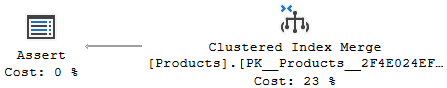
Clustered Index Merge

I’m guessing nobody will be surprised to see an operator called Clustered Index Merge at the heart of this execution plan. We are, after all, looking at an execution plan for a MERGE statements. So no surprise here.

However, there is not a 100% guarantee that a MERGE statement will always result in an execution plan with a Clustered Index Merge or Table Merge operator. I have seen cases where the optimizer created an execution plan with one or more Insert, Update, and/or Delete operators instead. And, conversely, I have also seen execution plans for statements other than MERGE that still end up using a Merge operator somewhere in the execution plan!

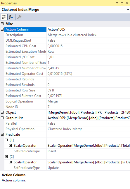But in this case, we get a pretty standard Clustered Index Merge operator. Let’s look at its properties to understand what it does.

The Action Column property should be simple to understand if you read all the previous explanations. Other sections go through great lengths to compute a value, representing insert, update, or delete, in the column Action1005. Here, the Clustered Index Merge operator is told to look at this exact column to determine what to do with each row it receives.

The more surprising property in the screenshot is the Predicate. This property is normally used to filter rows that can be disregarded. That’s not its function here. In fact, there is not really a Predicate property at all. You can call it a bug if you want to, or you can call it a feature; fact is that if you look in the underlying XML representation of the execution plan, you will see a property called SetPredicate. Or rather, you will see two of them. One with its SetPredicateType subproperty set to Insert, the other to Update.

If you expand the subnodes further than I have shown in the screenshot, you will see that the SetPredicate property with SetPredicateType Update assigns values to three columns: Price, ProductName, and Is_Deleted. For the columns that are not nullable, this is done with the special internal function RaiseIfNullUpdate, to ensure a run time error if the new value should be a null. The SetPredicateType Insert version has five assignments: copies of the three for update, plus assignments to ProductCode and TotalSold.

It is now obvious what this operator does: for each row it reads, it looks at the action column to determine whether the current row should be deleted, updated, or inserted. And when it needs to be inserted or updated, it uses one of the two sets of assignments in the SetPredicate property to determine the new values.

Finally, it returns a row to its parent operator, with all columns in the Output List property. Though not visible in the screenshot, you’ll find if you check the execution plan yourself that not only a few columns and the internal columns Action1005 and Expr1017 are returned to the parent, but also two columns named ProductCode_OLD and ProductName_OLD. When an internal column in an execution plan is the same as a column in a table, but without the table prefix and with “_OLD” appended, you know that this column is used to store the value that column had before an operator (such as in this case the Clustered Index Merge) modified its value in the actual table.

Assert

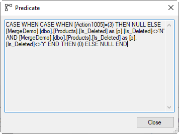The Assert operator here is used to verify a constraint. To see what exactly it checks, we need to look at its Predicate property. It returns NULL when nothing is wrong, or an integer value when something is bad and the query should rollback and return an error.

Unsurprising, the expression is again hard to parse due to all the prefixes, repeated aliases, brackets, and parentheses. Here is the simplified version:

CASE WHEN CASE WHEN Action1005 = 3
               THEN NULL
               ELSE p.Is_Deleted <> 'N'
               AND  p.Is_Deleted <> 'Y'
          END 
     THEN 0
     ELSE NULL
END;

We see a nested CASE in an unusual form. The result of the nested CASE is the entire input for the WHEN of the outer CASE. Which means that the nested CASE apparently returns a Boolean. Let’s review this nested CASE first.

When the action column is 3, the Clustered Index Merge has just deleted a row. In that case a null is returned, representing the Boolean value Unknown. For other cases (inserts and updates), the ELSE clause evaluates to the Boolean result of p.IsDeleted <> ‘N’ AND p.Is_Deleted <> ‘Y’. This is False is Is_Deleted is Y or N, Unknown if it is null, and True otherwise.

So all in all, the nested CASE returns False if we updated or inserted a row with an Is_Deleted value that is equal to Y or N (the values allowed by the CHECK constraint); it returns Unknown if we didn’t update or insert a row, or if we updated or inserted a row with a null value for Is_Deleted; and it returns True is we inserted or updated an Is_Deleted value that the CHECK constraint doesn’t allow.

Since this is the input to the WHEN of the outer CASE, it is the situation where True is returned that matters. That is when an update or insert was executed with an Is_Deleted value that is not null, and that violates the CHECK constraint. Then, and only then, the outer CASE of the Assert’s Predicate property returns 0 (zero), which will abort and rollback execution with a run-time error. In all other cases, execution continues.

Index maintenance

The fourth and final section of the execution plan is included for optimized maintenance of the nonclustered index that we have defined on the Products table. Not by execution an explicit CREATE INDEX statement, but by declaring a UNIQUE constraint on the ProductName column. For both PRIMARY KEY and UNIQUE constraints, SQL Server creates an index by default. And for a UNIQUE constraint, that index will be default be a nonclustered one.

The Clustered Index Merge has already changed data in the clustered index. If we leave it at that, we would get inconsistency. So we use, in this case, a (nonclustered) Index Update as well, to keep the nonclustered index in sync. The other operators in this section are there to optimize the performance of this process.

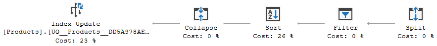
Split, Sort, and Collapse

The combination of Collapse, Sort, and Split operators you see here is very common when nonclustered indexes are maintained. It is not specific to plans for MERGE queries, so I will only describe it at a very broad level here.

Still following the right-to-left order of data travelling through the execution plan, the first operator to look at is Split. This operator looks at the action column to determine what to do. If an input row is an insert or delete, it is passed unchanged. If an input row is an update, it is transformed into two new rows: a delete of the old data, followed by an insert of the new data. The internal columns we previously saw that have “_OLD” at the end of their name are used here to construct the row with the deleted data.

The result of the Split operator is then (in the standard pattern, I’ll get to the Filter that is extra here shortly) sorted by the index key of the nonclustered index. That by itself is already a nice and simple way to gain some performance when updating the index. But in this case, it is also needed to ensure correct operation of the final element in this pattern.

The Collapse operator looks for immediately adjacent rows in its input that are a delete and an insert for the same key value, and replaces them with an update. Note that these are not the exact same row combinations previously created by the Split. The Split was used to break an update for a specific ProductCode into a delete and insert for that ProductCode; the Collapse creates updates to replace a delete and insert combination for the same ProductName.

The Split / Sort / Collapse pattern starts with a set of modifications that includes changes to the index key (and therefore requires data to be moved to a new location in the index); and transforms it into a set of changes that, as much as possible, uses in-place modifications of non-index columns. Combined with being able to process rows in order, this saves a lot of work when actually updating the index.

Filter

In this specific case, there Split / Sort / Collapse pattern has a Filter operator in between its elements. The reason for that Filter operator is to save even more work.

The Predicate property of this Filter is very simple: NOT Expr1017. Expr1017 is a Boolean internal column, holding the weirdly transformed and materialized equivalent of Expr1014. And Expr1014, computed in Compute Scalar #10 was set to True if the Merge had to update the row, but with a new ProductName value that is actually the same as it already was. Either because the update was only for Is_Deleted, or because NewProductName was null in the staging table, or because it was there but actually the same as in the Products table.

The NOT Expr1017 on this Filter means that all rows that have updated ProductName to exactly what it was are removed from the set here. What remains are inserted rows, deleted rows, and updated rows that actually changed the value of ProductName. So in plain English, this Filter simply removes updates that didn’t change the indexed column, since these were no real changes anyway. They won’t affect the nonclustered index.

I have to admit that I do not know why this is done after splitting the rows. I see no logical reason why this operator could not be moved to between the Clustered Index Merge and the Split, which would reduce the work for the Split operator a bit.

Index Update

Finally, after the updates needed to keep the nonclustered index consistent are optimized as much as possible, they are processed by the Index Update operator. The name of this operator is perhaps a bit misleading. I am not sure why, but SQL Server does not have a separate Index Merge operator. When index data needs to be changed and the changes can be a combination of inserts, updates, and deletes, it simply uses the standard Index Update operator.

My guess is that this is because index maintenance for any update statement is almost always optimized with a Split / Sort / Collapse pattern. Even if the input to this pattern is only updates, the split changes these to inserts and deletes and the collapses then replaces some of these with (new) updates. So the input to the Index Update operator will always be a combination of inserts, updates, and deletes.

And indeed, the Index Update operator does have an Action Column property that lists the column to look at in order to determine whether a row describes an insert, an update, or a delete in the nonclustered index. Note that even though this is still the same column (Action1005) we saw in use in the rest of the execution plan, the value in this column has been changed by the Split and Collapse operators.

Conclusion

Looking at the details of an execution plan for a MERGE query can be interesting and enlightening. Even if you always avoid using MERGE in your production code (which might be a pretty good idea), understanding how SQL Server processes this internally can still help you recognize and understand additional patterns in other execution plans.

That concludes part 11 of the plansplaining series. Many thanks to Andy Yun (B|T) for suggesting this topic. Do you also have a topic you would like to see me cover? Let me know, and I’ll add it to my list!