We’re already at part 31 of the plansplaining series. And this is also the third part in my discussion of execution plans for cursors. After explaining the basics, and after diving into static cursors, it is now time to investigate dynamic cursors. As a quick reminder, recall that a static cursor presents data as it was when the cursor was opened (and does so by simply saving a snapshot of that data in tempdb), whereas a dynamic cursor is supposed to see all changes that are committed while the cursor is open. Let’s see how this change in semantics affects the execution plan.

DYNAMIC FORWARD_ONLY cursor

The code below is almost identical to the sample code in the previous post. The only change is the cursor type: DYNAMIC instead of STATIC.

DECLARE MyCursor CURSOR
                 GLOBAL
                 FORWARD_ONLY 
                 DYNAMIC
                 READ_ONLY
                 TYPE_WARNING
FOR
SELECT     soh.SalesOrderID,
           soh.OrderDate,
           sod.SalesOrderDetailID,
           sod.OrderQty,
           sod.ProductID,
           p.ProductID,
           p.Name
FROM       Sales.SalesOrderHeader AS soh
INNER JOIN Sales.SalesOrderDetail AS sod
   ON      sod.SalesOrderID        = soh.SalesOrderID
INNER JOIN Production.Product     AS p
   ON      p.ProductID             = sod.ProductID
WHERE      soh.SalesOrderID  BETWEEN 69401 AND 69410
AND        sod.OrderQty           >= 10
ORDER BY   p.ProductID;

OPEN MyCursor;
FETCH NEXT FROM MyCursor;
FETCH NEXT FROM MyCursor;
CLOSE MyCursor;
DEALLOCATE MyCursor;

As before, you have two options to inspect the execution plans for this batch. You can execute the queries (all at once or one at a time) while requesting the execution plan with run-time statistics, or you can request the execution plan only. In the latter case, you only need to do this for the DECLARE CURSOR statement. I have chosen the latter option, because that is the only method that gives access to the properties in the Keyset pseudo-operator.

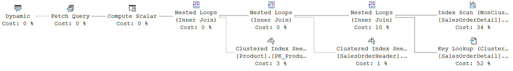
(Click on the picture to enlarge)

As you can see, there is no Population Query at all in this case. Just a Fetch Query. And indeed, if you step through the code while requesting execution plans with run-time statistics, you will see that no execution plan is used for the OPEN CURSOR statement, and each FETCH statement returns a copy of the Fetch Query sub-plan above.

Fetch Query

If you look at the sub-plan for the Fetch Query above without taking the cursor context into account, then you will probably wonder what drugs the optimizer was on when it created this plan. The top right Index Scan on SalesOrderDetail uses the index on ProductID, with the Ordered property set to True. And yes, this does avoid the need to have a Sort operator – as you can see, there are none in this execution plan. But it comes at a high price. The Index Scan has to read through all 121,317 rows in the index to return the just 176 (estimated) rows that match the Predicate that filters on SalesOrderID.

These are then passed into a Key Lookup, and because that Key Lookup has an additional Predicate property to filter on OrderQty >= 10, only 59 (estimated) rows remain from the 176 (estimated) executions of this operator. Please note that the numbers that you see in the properties list of this Key Lookup are very confusing and misleading in this case, due to this bug that, unfortunately, still has not been fixed yet.

The end result is that, indeed, all results are produced, without ever having to sort the data. But this comes at the price of having to read all 121,317 rows from the index on ProductID, and then having to do an estimated 176 Key Lookups. That is so much more I/O than the execution plan that we saw in the previous episode of this series, that the total estimated cost of this plan (1.04495) exceeds the estimated cost of the plan for the static cursor or for the cursor-less execution of the query (0.056249) by quite a bit. This plan, is, in fact, over 18 times as expensive! And that is for just a single execution. In reality, this plan will execute for each FETCH statement, whereas for the static cursor, it executed only once.

However, that is all without taking into account that this is actually a Fetch Query. And those execute different. To get a better insight in how the execution plan for the Fetch Query really works, it is in this case helpful to actually run the code, and request the execution plans with run-time statistics. If you do that, you will see the following plans returned:

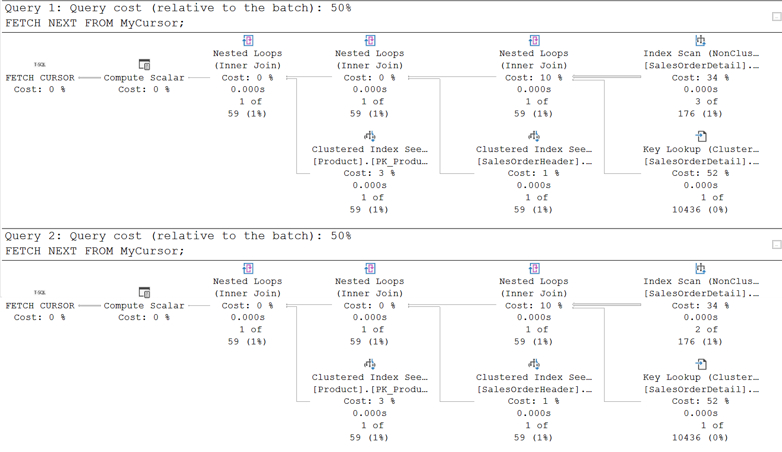
(Click on the picture to enlarge)

Now, hold it. Don’t start shouting at me that I am wasting space in this blog by posting two identical copies of the same plan. Look closer. Are they really identical? Look specifically at the numbers below the top right Index Scan, that reads SalesOrderDetail, through an index on the ProductID column. Why is the Actual Number of Rows equal to 3 for the first FETCH statement, but only 2 in the second? And, not visible in the screenshot above, if you look at the properties of that Index Scan, you’ll see that the Actual Number of Rows Read differs even more: 5,527 for the first FETCH statement, and only 3,267 for the second. What is the reason for these differences?

First FETCH

For the first FETCH, the explanation is actually quite simple. You only need to realize that a FETCH statement doesn’t keep requesting rows. It stops as soon as the first row is returned. So what happens is that the Index Scan starts reading from index IX_SalesOrderDetail_ProductID, in order, until it finds a row that meets the Predicate (SalesOrderID BETWEEN 69401 AND 69410). When does that happen? If you are patient enough, you can find that out by running the query below:

SELECT  *
FROM    Sales.SalesOrderDetail AS sod WITH (INDEX = IX_SalesOrderDetail_ProductID)
OPTION (MAXDOP 1);

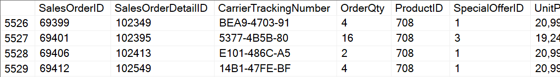
This returns all rows from SalesOrderDetail, in order of the IX_SalesOrderDetail_ProductID index. So you can scroll through the results and look yourself which rows meet the Predicate. To save you some time, I have done that for you. The first row that will be returned is row number 2,478 (see screenshot below).

This row gets returned to the Nested Loops, the Key Lookup reads the rest of the data, and then rejects it, because the OrderQty is 8, which fails the OrderQty >= 10 test. The Index Scan then instantly returns the next row, but again, the Key Lookup rejects it because of a too low OrderQty. After that, Index Scan once more skips through many rows with a SalesOrderID that falls outside the requested range, until it hits row number 5,527:

This row is also passed through the Nested Loops into the Key Lookup, and now we find an OrderQty of 16, which is sufficient to be included in the results. This row is then passed through the other Nested Loops and Clustered Index Scan operators, and then finally returned to the client. At that point, FETCH is done. And we see that all the numbers match. The Index Scan has read 5,527 rows, passed 3 to Nested Loops, Key Lookup was executed 3 times, and it only returned a single row.

Second FETCH

But because the cursor is still open, the execution plan is not closed. It remains active, in a paused or suspended state. Once the next FETCH statement starts, the plan is not restarted from scratch. It simply continues where it left.

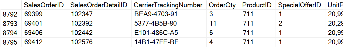
So we would expect that it first reads row 5,528 (visible in the screenshot above), passes it through Nested Loops into Key Lookup, which then rejects it because of the too low OrderQty.

After that, the Index Scan would skip rows 5,529 until 8,792, based on the Predicate on SalesOrderID, but row 8,793 would then be returned again.

This row does qualify based on OrderQty as well, so it is passed through the rest of the execution plan and returned to the client. Let’s see if all the numbers match.

We read rows 5,528 until 8,793. That is a total of 3,266 rows read. We returned two of them to the Nested Loops, which caused 2 executions of Key Lookup, returning 1 row, which in turn caused 1 execution with 1 row returned for both of the Clustered Index Seek operators. Do those numbers all match in the execution plan?

Sadly, they don’t. The Index Scan reports 3,267 rows read. One more than I computed. It did indeed return 2 rows. And yet, the Key Lookup has not 2 but 3 executions! The number of rows returned from this operator is once more as expected: just 1. And if we look at the two Clustered Index Seek operators, we see that they, too, do return the expected 1 row, but with 2 instead of 1 as their Number of Executions.

Why all these differences? My theory is that this is necessary because of some internals of how SQL Server reads data. When row 5,527 was read, as the last row accessed for the first FETCH, the internal read position was already advanced to the next row to be read, row 5,528. So when the second FETCH started, the Index Scan was already ready to return that row. However … that could potentially cause incorrect results!

Remember, a dynamic cursor must also return rows that are added after the cursor is open. Let’s imagine that I run the first FETCH. Then, from another connection, you add a row, with SalesOrderID 69403, ProductID 711, and OrderQty 13. That row would then be inserted between rows 5,527 and 5,528 in the index on ProductID. It is added after the cursor is opened, but because the cursor is dynamic, we need to return it. But the Index Scan has already advanced its read position to the original row 5.528, past this new row. We would miss it, and that would be an incorrect results bug.

To make sure that we do not miss a row that might be inserted in between the last row returned and the current internal read position, SQL Server actually starts the second query by re-reading the last row read, instead of instantly advancing. That accounts for the 1 extra row read by the Index Scan. And since that was a qualifying row, it also accounts for the 1 extra execution of the Key Lookup and the two Clustered Index Scans. But … now we have a new inconsistency! Now the number of rows returned by each operator that I expect is one more than what is actually reported by the execution plan!

So, what is the explanation for this new inconsistency? My theory is that Microsoft specifically coded the operators to not count the row that is read first, that is only read for the purpose of readjusting the internal read position. My guess is that they decided to keep this row out of the counters to prevent confusion when an execution plan is casually inspected, but were not aware that, by doing so, they caused more confusion for those who look deeper and actually inspect all properties.

Unfortunately, none of all this special magic is exposed in any way in the execution plans. Well, except indirectly, through the numbers that don’t seem to match up until you realize that each FETCH starts by re-reading the last row, which is recorded in all counters except Actual Number of Rows.

DYNAMIC SCROLL cursor

The discussion above was all for a FORWARD_ONLY cursor, which is relatively easy, because it supports FETCH NEXT only. A SCROLL cursor is much more complex, because it allows us to jump around at will inside the result set of the cursor. And all that while still also observing the DYNAMIC property, which means that rows inserted, deleted, or updated after the cursor was opened should still be reflected in the results.

So here is a bit of sample code that, based on the same query, showcases all the supported FETCH commands:

DECLARE MyCursor CURSOR
                 GLOBAL
                 SCROLL 
                 DYNAMIC
                 READ_ONLY
                 TYPE_WARNING
FOR
SELECT     soh.SalesOrderID,
           soh.OrderDate,
           sod.SalesOrderDetailID,
           sod.OrderQty,
           sod.ProductID,
           p.ProductID,
           p.Name
FROM       Sales.SalesOrderHeader AS soh
INNER JOIN Sales.SalesOrderDetail AS sod
   ON      sod.SalesOrderID        = soh.SalesOrderID
INNER JOIN Production.Product     AS p
   ON      p.ProductID             = sod.ProductID
WHERE      soh.SalesOrderID  BETWEEN 69401 AND 69410
AND        sod.OrderQty           >= 10
ORDER BY   p.ProductID;

OPEN MyCursor;
FETCH NEXT FROM MyCursor;
FETCH NEXT FROM MyCursor;
FETCH PRIOR FROM MyCursor;
FETCH LAST FROM MyCursor;
FETCH FIRST FROM MyCursor;
FETCH RELATIVE 7 FROM MyCursor;
FETCH RELATIVE -3 FROM MyCursor;
--FETCH ABSOLUTE 4 FROM MyCursor; -- The fetch type Absolute cannot be used with dynamic cursors.
CLOSE MyCursor;
DEALLOCATE MyCursor;

I will not include a screenshot of the execution plan for this version of the code, because the plans are all exactly identical to the execution plans we have seen before (except for some of the run-time statistics, if you actually run the code).

The behavior of each of the FETCH options does change, though. This is very hard to investigate through the execution plans (although the Actual Number of Rows property and some other properties might provide a clue). I found that I made more progress with analyzing how each FETCH type behaves by running a single FETCH statement in a transaction, with repeatable read isolation level, and then checking which rows and which key values were locked. That way I was able to figure out which rows were touched in each case. To figure out the order, I then locked one of those rows from another connection, repeated the process, and checked which locks were already granted to the FETCH before it started to wait on the competing lock.

Does that sound like a lot of work? Well, it is. And I won’t bother you with all the details. Instead, I will provide a quick summary of how I think each FETCH type works.

FETCH FIRST

Execution of a FETCH FIRST completely disregards the current position of the cursor, and by extension the current read position of all scan and seek operators. It resets everything, then starts executing the operators until a row is returned. At that point, execution is stopped. The internal position of the seek and scan operators is on the row just after the last row read.

FETCH LAST

Execution of a FETCH LAST also completely disregards the current position of the cursor, and by extension the current read position of all scan and seek operators. It resets everything, then starts executing the operators until a row is returned. However, in this case, the read direction of seek and scan operators is reversed. So an operator that has its Ordered property set to FORWARD will actually run as if the Ordered property is BACKWARD. (And vice versa). Note that this is not visible in the execution plan!

Once a matching row is found, the internal read positions of all seek and scan operators will be on the row before that row. That would be a problem, because other FETCH operators expect the internal read position to be after the row just returned. In order to fix this, the row that is found is not returned. Instead, the cursor keeps processing (still in backward direction) until another row is found. Then the direction is reversed, and the cursor once more processes, until the first row found, the last row, is found again. Now it is returned, and because the last reads were in the regular direction, the internal position of the seek and scan operators will be as expected.

FETCH NEXT

This works the same for a SCROLL cursor as for a FORWARD_ONLY cursor, so exactly as described in the main text: it first re-reads the row that was returned by the last FETCH statement, does not return it (and does not count it in the Actual Number of Rows counters, but does still update all other counters), and then continues with the execution plan as expected, until a row is returned and execution is stopped.

FETCH PRIOR

The FETCH PRIOR is where it really gets complex. It combines elements of the FETCH LAST process (especially the reversed read order) with elements of FETCH NEXT (starting by re-reading the last row read instead of starting at the internal position). Putting it all together, FETCH PRIOR first re-reads the last row read, but with the read direction reversed. So this gives us the same row again, but the internal position for scan and seek operators is now just before that row. Regular processing starts, until a row is found. That would be the prior row, but we once more have the problem that the internal read positions are now before it, instead of after. So, just as for READ LAST, processing continues in reverse direction until yet another row is found, and then resumes in forward direction, back to the row we already found as the prior row. Now all internal positions are as expected, and the row can be returned.

FETCH RELATIVE

The operation of a FETCH RELATIVE depends on whether the number given is positive (to progress in the normal read direction of the cursor), or negative (to effectively move back).

For a positive number, the behavior is similar to that of FETCH NEXT. Which makes sense, because FETCH NEXT can be seen as a shorthand for FETCH RELATIVE 1. So this means that for e.g. FETCH RELATIVE 3, the cursor will first re-read the last row read, then read the next three rows, skipping the first two and returning the third.

For a negative number, FETCH RELATIVE behaves similar to FETCH PRIOR: it first re-reads the last row read, with reverse read direction. It then reads and skips an equal of rows equal to the absolute value of the argument plus one (so e.g. FETCH RELATIVE -4 would read and skip five rows, all the time reading backwards in the cursor). Then it sets the read direction to forward again, for a final read of the row to be returned.

Correct?

As I said above: the above is how I think the various FETCH options work. I am absolutely not sure. I have described this based on observations, by checking which rows were locked by executing a FETCH statement, and in what order. After observing that reality, I tried to explain why it works this way. I am not very happy with this explanation myself. I feel I am missing something.

It seems that some statements, especially those that read “backwards”, do extra work to ensure that the internal positions for seek and scan operators are at the “next” row after the row returned. And that would make sense if there were any operations where that position would be relevant. But it isn’t, because, as far as I can tell, all operations always start by re-reading the last returned row. Which resets those internal positions anyway.

I feel that there must be another explanation. I just don’t know what it is. If you do, then please leave a comment, so I can update this post!

Concurrency

For DYNAMIC cursors, all three concurrency options are supported. Remember, you can set them by changing the READ_ONLY keyword in the DECLARE CURSOR statement to OPTIMISTIC, or to SCROLL_LOCKS. Choosing either of the latter two options allows you to update or delete from tables referenced in the cursor’s SELECT statement by using the WHERE CURRENT OF clause of the UPDATE and DELETE statements.

The concurrency option is directly visible in the execution plan, in the properties of the Dynamic pseudo-operator. The screenshot on the right is for a dynamic cursor with concurrency option DYNAMIC. As you can see, the Cursor Concurrency property is now set to “Optimistic”, whereas it was “ReadOnly” in the original example. At this point, you might expect that the third possible value of this property is “ScrollLocks”. But that is not the case. Change the cursor’s concurrency option to SCROLL_LOCKS, and the Cursor Concurrency property will read “Pessimistic”.

For both types of cursor, the execution plan also changes a bit. I will look at those changes, and their reasons, in a later post, when I’ll also describe the execution plans for UPDATE and DELETE statements that actually use the WHERE CURRENT OF clause.

Summary

A DYNAMIC cursor does not use a Population Query. It has only a Fetch Query. This is an execution plan that appears to read all rows from start to finish. But in reality, the execution is paused after a FETCH statements returns data, and the next FETCH statement basically resumes from where we were.

For reasons that are not entirely clear, FETCH NEXT and FETCH RELATIVE with a positive number first re-read the row last returned, before moving further. FETCH statements that read in backwards order (PRIOR and RELATIVE with a negative number) do the same, but in backwards direction, and they then also read even one more row, before backtracking to the row they have to return. That same “reading one more row and then backtracking” is also done by FETCH LAST.

If you don’t specify a cursor type, SQL Server defaults to DYNAMIC if it is supported for the query used. I am not happy with this default, because most applications that need a cursor do not need to see all changes. A STATIC cursor would often be better, and is almost always the better choice for performance! That said, I have an opinion on using default options anyway. Just type those few extra keystrokes to make your code self-documenting and avoid all unclarity!

If your application needs a cursor that sees all concurrent changes, then you have no other option but to use a DYNAMIC cursor. And if you need to access the rows from that cursor in random order, they you will also need to use SCROLL instead of FORWARD_ONLY, and take the extra performance hit on all FETCH statements that use a backwards direction.

In the next post in this series, I’ll look at KEYSET cursors. As always, please let me know if there is any execution plan related topic you want to see explained in a future plansplaining post and I’ll add it to my to-do list!