Welcome back to my plansplaining blog series, where I dive deep into the details of non-obvious execution plans. This part is also a sort of follow up on my post from two weeks ago, when I wrote about the structure and usage of XML indexes, and had to admit that I had not been able to come up with good use cases for all types of secondary XML index.

That very same day, I received an email from Mikael (Micke) Eriksson, who pointed me to this question and answer on Stack Exchange for Database Administrators. I then modified that example a bit, to come up with an execution plan that I consider interesting enough that I want to describe it here.

The setup

The change to the setup is only minimal. I created a permanent table, rather than the temporary table in the Stack Exchange post, and renamed one of the columns. And I added a few extra indexes – where the original post creates only a primary XML index and a PATH secondary XML index, I decided to also add a VALUE and a PROPERTY secondary XML index, to give the optimizer all possible options.

Here is the modified setup script:

DROP TABLE IF EXISTS dbo.TestXML;
GO

CREATE TABLE dbo.TestXML
    (PK        int IDENTITY PRIMARY KEY,
     SomeData  varchar(100),
     XmlColumn xml);
GO

-- Executes 100,000 times. Do NOT enable execution plan plus run-time stats here!!!
-- One of the values in the XML below is a random value between 0 and 999.
DECLARE @RndNumber varchar(100) = (SELECT CAST (CAST (RAND () * 1000 AS int) AS varchar(100)));

INSERT INTO dbo.TestXML
VALUES ('Data_' + @RndNumber,
        '<error application="application" host="host" type="exception" message="message" >
  <serverVariables>
    <item name="name1">
      <value string="text" />
    </item>
    <item name="name2">
      <value string="text2" />
    </item>
    <item name="name3">
      <value string="text3" />
    </item>
    <item name="name4">
      <value string="text4" />
    </item>
    <item name="name5">
      <value string="My test ' + @RndNumber
        + '" />
    </item>
    <item name="name6">
      <value string="text6" />
    </item>
    <item name="name7">
      <value string="text7" />
    </item>
  </serverVariables>
</error>');
-- Repeat this batch 100,000 times
GO 100000

-- Create primary XML index and all three secondary XML indexes
CREATE PRIMARY XML INDEX PXML_test_XmlColum1 ON dbo.TestXML (XmlColumn);
CREATE XML INDEX IXML_PATH_test_XmlColumn2 ON dbo.TestXML (XmlColumn) USING XML INDEX PXML_test_XmlColum1 FOR PATH;
CREATE XML INDEX IXML_PROPERTY_test_XmlColumn2 ON dbo.TestXML (XmlColumn) USING XML INDEX PXML_test_XmlColum1 FOR PROPERTY;
CREATE XML INDEX IXML_VALUE_test_XmlColumn2 ON dbo.TestXML (XmlColumn) USING XML INDEX PXML_test_XmlColum1 FOR VALUE;
GO

The query

In the Stack Exchange post, several queries were executed, before and after creating the XML indexes. I will stick to just a single of those queries. And I have (for now!) added a query hint to force row mode execution. Since the post was from 2012, when batch mode on rowstore did not exist yet, that hint was not needed in the original post. I obviously also got rid of the SELECT *, simply because I refuse to show bad examples.

So that means that this is the query I executed:

SELECT      PK, SomeData, XmlColumn
FROM        dbo.TestXML
CROSS APPLY XmlColumn.nodes ('/error/serverVariables/item[@name="name5" and 
                                                          value/@string="My test 600"]') AS a(b)
OPTION (USE HINT ('DISALLOW_BATCH_MODE'));

This returns all the rows that have been generated with 600 as the random value. Statistically speaking, we can expect approximately 100 rows returned. But in reality, the number of rows returned can be less or more than that, due to fluctuations in randomness. In my case, the result set includes 118 rows.

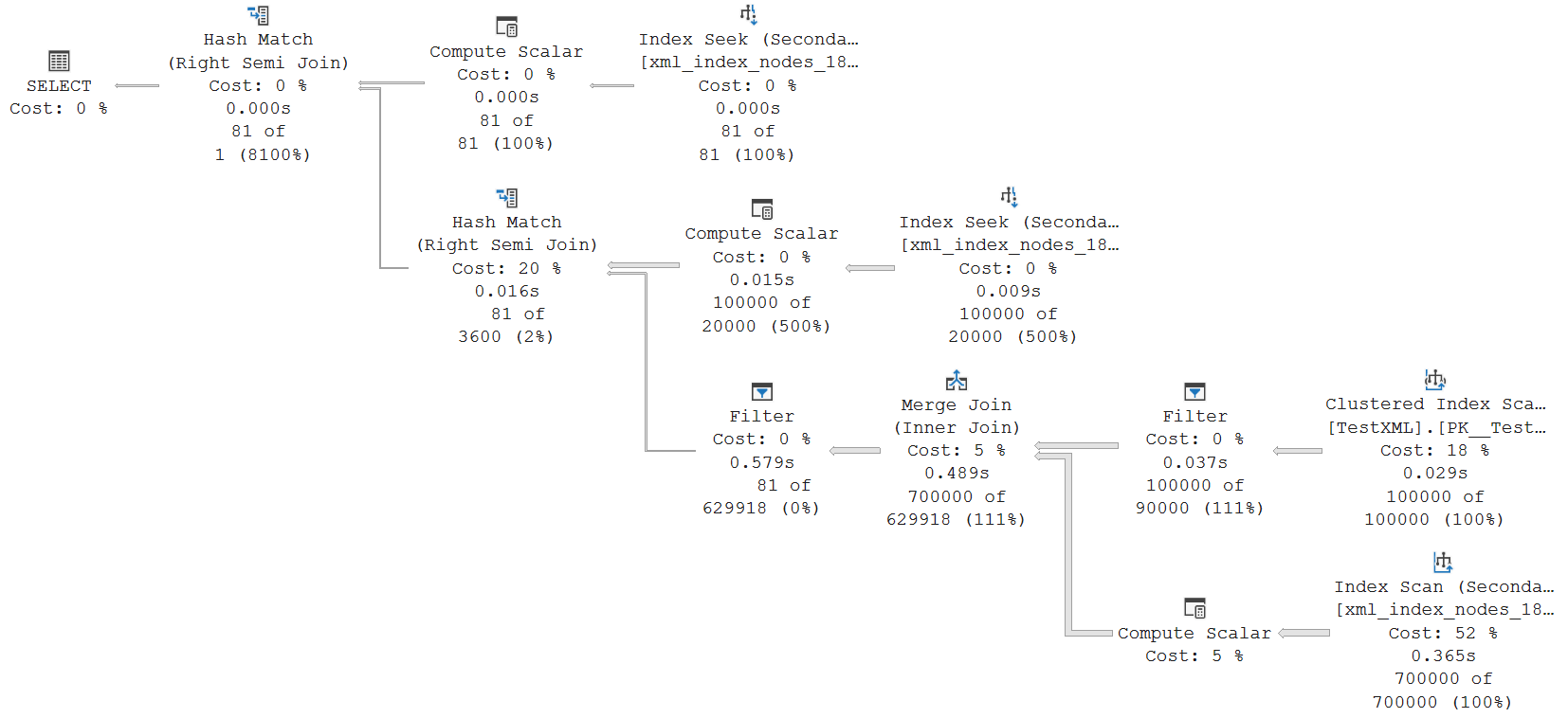
But I really don’t care about the results of this query anyway. I want to look at the execution plan. So below is the execution plan that I got when I ran this on my SQL Server 2025 instance, with Node ID values added in red to make it easy to refer to specific operators in the rest of this post.

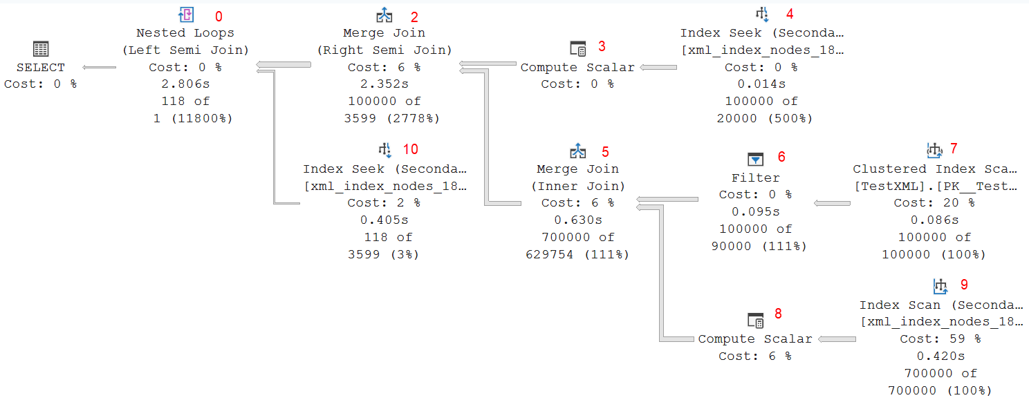
What I find interesting in this execution plan is that each of the three secondary XML indexes is used. Index Seek 4 reads from the VALUE index, Index Scan 9 from the PROPERTY index, and Index Seek 10 from the PATH index. You might say that this would have been the perfect illustration for my previous post!

Row mode execution

Let’s walk through this execution plan, step by step. The order might not seem logical, but bear with me.

Clustered Index Scan #7

As I explained in a previous post, XML indexes are actually just clustered and nonclustered on a collection of data that is obtained by shredding the content of the XML column, plus a reference to the original row in the form of the primary key value. Any query that returns other data from the table, such as the sample query, needs to join the data found from the XML indexes back to the clustered index by using that primary key value.

That is what this Clustered Index Scan does. The optimizer has in this case chosen to fetch all rows and then later join this to the data from various other seeks and scans on the XML index that perform the selections indicated in the XQuery expression. I’m not sure why this choice is made. After all XML-based selections are done, we are left with just 118 rows. The optimizer expects even less: just a single row. I think an execution plan that first does all the XQuery selections in the XML indexes and then does a Clustered Index Seek on the primary key value for just the remaining estimated 1 (actual 118) rows would be cheaper. But that is not what the optimizer decided. All 100,000 rows from the original table are read and returned by this Clustered Index Scan. Note that the Ordered property is set to True, so the optimizer forces the run-time engine to use an ordered scan. The data is returned in logical order of the clustered index key, the primary key column of the table: PK.

Filter #6

The Filter operator then removes all rows for which the XmlColumn holds a NULL value. That seems like a smart thing to do. After all, if the XmlColumn is NULL, then the XQuery expression can never be true, and this row won’t qualify. So let’s remove it as soon as possible.

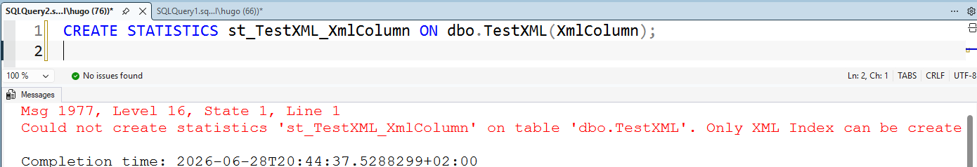
I have two questions here, though. First, what exactly made the optimizer decide to estimate that 10% of the data would be removed by this filter? You might think that the optimizer decides this based on statistics on the XmlColumn. But that is not the case. No such statistics exists, even though I have the AUTO_CREATE_STATISTICS option turned on. SQL Server will not create statistics on an XML column, ever. Not automatically, when it would be helpful. And not when explicitly requested either!

So, in the absence of statistics, the estimate of 10% NULL values in this column is simply a hardcoded number, completely unrelated to any reality. Whether the actual data has 0% NULL values (as in this example), or 99%, the optimizer will always assume it’s 10%.

The second question I have when I see this Filter operator is: why is this predicate not pushed into the Clustered Index Scan? I have no real answer for this. Other than my wild guess that this is a limitation of the product. Apparently, NOT NULL tests on XML columns cannot be pushed into a Clustered Index Scan.

Either way, the final result of this branch of Clustered Index Scan #7 and Filter #6 is that we now have a recordset that includes the PK, SomeData, and XmlColumn columns for all 100,000 rows in the table. We’ll later see how this is used.

Index Scan #9

Here, we see the first operation that targets one of the XML indexes. The PROPERTY index in this case. This is the relevant part of the properties:

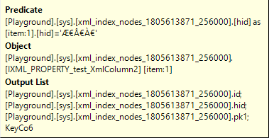
So you see in the Object property that, indeed, the PROPERTY secondary XML index is the target of this Index Scan. And the Predicate property shows that it only returns rows with the hid column equal to the encoded value ƀŀ. By opening a DAC connection and querying the nodes table, I was able to reverse engineer that this value ƀŀ is the encoding for the node <error><serverVariables><item>. There are seven such nodes in each of the 100,000 XML values, so that is why this Index Scan returns 700,000 rows.

The conclusion is that this Index Scan is where the first part of the XQuery expression is evaluated: the path /error/serverVariables/item. Nothing is done here with the rest of the expression: [@name=”name5″ and value/@string=”My test 600″]. We’ll find those elements in other operators in the execution plan.

The Index Scan then returns four columns from this nonclustered index: id, hid, pk1, and KeyCo6. I described the first three in my blog post about XML indexes. The last one is weird, because no column of that name exists in the node table, or in the PROPERTY index. However, since this KeyCo6 column is also not referenced anywhere in the rest of the execution plan, I decided not to worry about it.

Unfortunately, the PROPERTY index is not very efficient for the type of search done here. We are searching for a specific value in the hid column. This column is the second indexed column of the PROPERTY index, which means we have to scan the entire table. And this is confirmed in the properties of this operator: it had to read 3,5 million rows to find the 700,000 required rows.

It is strange that the PATH index is not used instead. After all, this is the index that has the hid column as its leading column, so an Index Seek on that index would find the 700,000 required rows without reading any other data. The columns that we need to return, as shown in the Output List property, are id, hid, and pk1 (I’ll pretend KeyCo6 does not exist). Well, we have hid as one of the indexed columns in the PROPERTY index, and both id and pk1 are included because they are the reference to the primary XML index, the clustered index on the node table. So I believe that the optimizer made a suboptimal choice here. An Index Seek on the PATH index, with Seek Predicates set to hid = ‘ ƀŀÀ€’, would have returned the 700,000 rows with id, hid, and pk1, at a lower number of logical reads.

This Index Scan also has its Ordered property set to True. This means that rows are returned in the order of the indexed columns. For a PROPERTY index, that is pk1, hid, value. In the context of this specific execution plan, it is important to know that all rows from the node table that match the specified path /error/serverVariables/item (seven per row in the base table) are returned in order of pk1, the table’s primary key.

Compute Scalar #8

This Compute Scalar returns the same 700,000 rows as Index Seek #9. But of the original input columns, only id and pk1 remain. The hid and KeyCo6 columns are dropped from the rows. Instead of that, one new column is added: Expr1025. This column is computed using the “getdescendantlimit” internal function, with id as its input parameter. This returns the id of the first node that is not a direct or indirect child of the input node. So with the id of the name5 element passed in, the value in Expr1025 would be the id of the name6 node for all the input rows.

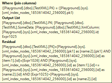
Merge Join #5

The two inputs described above are not joined using a Merge Join operator, performing an Inner Join Logical Operation. The Where (join columns) property shows that the join criterium is that the PK value from Filter #6 (which is the primary key of the test table) must be equal to the pk1 column from Compute Scalar #8 (the column from the nodes table that ties the XML nodes to the rest of the table, using the primary key value). So this join criterium makes sense.

Because both inputs use an ordered scan on an index that has the join column as its leading column, the data in both inputs is sorted. Which means that a Merge Join is safe and cheap to use here. The optimizer also knows that there can’t be duplicate PK values in the upper input, so the Many to Many property is set to False, which means that the cheap one-to-many merge join algorithm can be used.

The output of this Merge Join is then the columns PK, SomeData, and XmlColumn from the table, plus id (the path to the /error/serverVariables/item node) and Expr1025 (the path to its last descendant, or rather the node after it).

At this point, all rows with a NULL value in XmlColumn  are excluded, as well as all rows with an XML value in that column that does not include any /error/serverVariables/item path. Granted, that rules out exactly zero rows in this specific test data. But the optimizer can’t know that when it creates this plan, and the logic makes sense.

For the remaining rows, we have not yet checked the @name=”name5″ and value/@string=”My test 600″ expressions. But we do already know that the referenced @name attribute and the value node must be in the node table with an id somewhere between the id and Expr1025 columns from the Merge Join output.

These results are then one of the two inputs to Merge Join #2. Let’s now first look at the other input.

Index Seek #4

For this Index Seek, the optimizer has chosen to use the VALUE secondary XML index, with a Seek Predicates property that searches for specific values in two columns: the value column must be equal to name5, and the hid values must be the encoding of the value property of the name attribute in an element with pathname /error/serverVariables/item. The test data has seven such elements in each XML fragment, but only one of them has the value name5. So this Index Seek returns exactly one row from the node table for each row in the base table. And because we use an Index Seek on the full index key, this is done efficiently – the operator only reads those exact 100,000 rows.

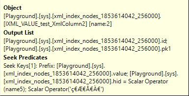
The data returned are just two columns: id (the path to the node that was found) and pk1 (the primary key from the underlying row in the base table).

The optimizer’s choice for the VALUE index seems to be arbitrary in this case. The VALUE index is on columns (value, hid). But there is also a PATH index, which is on the same columns, just in a different order: (hid, value). Since both columns are provided with an equality in the Seek Predicates, both would have been equally effective here.

Compute Scalar #3

Where Compute Scalar #8 looked down in the XML to find the id of the last child node for each found node, this Compute Scalar operator does the reverse: it uses the internal function getancestor, with input parameters id from the input row and a constant 1. This returns the id of the direct parent of the node that was found. So that would be the /error/serverVariables/item node.

Merge Join #2

The bottom input to this Merge Join is still in order of the primary key column – both its inputs were in that order, a requirement for the Merge Join to work, and Merge Join retains that order.

The top input is in order of the VALUE index that was read in Index Seek #4. So that would be in order of (value, hid). And for rows that have the same value in both these columns, the order would be further sorted by the primary key: (pk1, id). However, Index Seek #4 has a Seek Predicates that matches just a single (value, hid) combination. So all rows returned have the same value in those two columns, and that means that the secondary sort order by primary key is actually relevant. All rows have the same value and hid, and are then sorted by pk1 and id.

With both inputs effectively sorted by the primary key (PK in the base table, or pk1 in the node table), the Merge Join can indeed process the join based on the Where (join columns) property you see above. However, in this case, the algorithm is a bit less effective. SQL Server has to set the Many to Many property to True, because there might be duplicates in both inputs. (We know that there are none in the top input, but we know that because we have knowledge of the XML in the test data. The optimizer does not have this knowledge).

However, this Merge Join does not simply join on equality of the primary key. That is just the start. The full test that is applied before calling two rows from the two inputs a match is found in the Residual property. This is a bit hard to read, due to all the repeated brackets and full names. So let me break it down for you.

The first part of the Residual is simply a repeat of the join condition: PK from the bottom input must be equal to pk1 from the top input.

The second part then checks that the id value from the bottom input must be equal to Expr1026, the parent node from the name5 element from the top input. This ensures that a match is only considered a match is the name5 element that was found in the top input is actually in the /error/serverVariables/item found in the bottom input. So if an XML fragment does have a /error/serverVariables/item path, and does have a name5 element but somewhere else in the XML, then this extra test would ensure that this is not considered a full match.

Finally, the third and fourth part of the Residual then check the id column from the top input against the id and Expr1025 values from the bottom input. Remember, the latter indicate the first and last child elements of the /error/serverVariables/item path. So this is effectively another way to check that the name5 element found in the top input is in a child node of the /error/serverVariables/item element found in the bottom input. I think this check is redundant after we already checked that /error/serverVariables/item is the direct parent of name5, but it seems that Microsoft let it in anyway – better safe than sorry, I guess?

It is also important to notice that the Logical Operation of this Merge Join is a Right Semi Join. That means we’re effectively doing an EXISTS check. Rows from the “right” (bottom) input – those are the rows from the base table that have an element with pathname /error/serverVariables/item – are retained if there is at least one matching row in the left or top input. In other words, we now check that the previously found rows with an element with pathname /error/serverVariables/item have at least one child node in that path with @name=”name5″. There could be more, but that will not affect the results.

The returned columns are the same as from Merge Join #5: PK, SomeData, and XmlColumn from the table, plus id (the path to the /error/serverVariables/item node) and Expr1025 (the path to its last descendant, or rather the node after it).

Nested Loops #0

This Nested Loops join operator also does a semi join. A Left Semi Join, in this case. Which once more means an EXISTS check. The data returned from Merge Join #2 will be kept if a match is found in Index Seek #10, or rejected if not.

This Nested Loops then uses the Outer References property. That means that data from the top input is pushed into the bottom input to return only matching rows. We see that in this case four columns get pushed: the PK column from the base table, the id column that stores the encoded path to the /error/serverVariables/item node we found in the bottom right of the execution plan, and then matched against an @name=”name5″ element, the Expr1025 column that can be used to find the last child element of that node, and a new column, Expr1027. It is not clear where in the execution plan this column is computed, but it is then also not used in any way. So like the KeyCol6 column I saw before, I will pretend this column does not exist.

Index Seek #10

We already verified a lot of the criteria from the query. The rows we found must have actual XML data in the XmlColumn. That XML data must include a node /error/serverVariables/item, and that node must include an @name=”name5″ element. If we compare this to the original query, we see that one part is still missing: value/@MyString=”My test 600″. This is what we then expect to see in this last EXISTS test, Inner Join #0 into this Index Seek #10.

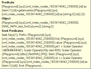
The Object property shows that, in this case, we are using the PATH index to search for matching rows. And the Seek Predicates then shows what we are searching for: the indexed columns hid and value must be equal to the encoded version of the path /error/serverVariables/item/value/@string, and the value “My test 600” respectively. Additionally, the pk1 column (remember that nonclustered indexes have the clustered index key as a kind of secondary index columns!) must be equal to PK, and the id column must be between the id column and Expr1025 from Compute Scalar #8. So we are looking for the same base table row, with a node that is a descendent of /error/serverVariables/item found in Index Scan #9 and then later already verified to have an @name=”name5″ element, and that child node must now meet the value/@MyString=”My test 600″ criterion.

The Predicate property then does an extra test to ensure that the id of the top input is the grandfather (getancestor with 2 as its second parameter) of the node found in Index Seek #10. This makes sure that we only return matches where value/@MyString=”My test 600″ is directly underneath the /error/serverVariables/item node, with no other nodes in between.

Recapture

So to recapture this entire execution plan, what we see is that the optimizer first gets all the data from the table where the XML column is not NULL. It then applies the filters from the XQuery string one at a time. It first finds all /error/serverVariables/item nodes. It then removes those that do not have an @name=”name5″ element, and the final step is to then also check for the presence of value/@MyString=”My test 600″.

With our knowledge of the test data, that order is not the most efficient. But we realty can’t expect the optimizer to know this. Remember, there are not even any statistics on the XML column!

We also saw that, in this specific case, each of the three secondary XML indexes was used. In one case, that seemed to be a rather arbitrary choice. And in another, the choice was in my opinion even suboptimal. But it did give me a great opportunity to show an execution plan that uses all three of these indexes!

Batch mode execution

Given the sheer size of the node table and its indexes, I had to add a hint to the query to ensure that the execution plan would use row mode execution. With tables of this size, the batch mode on rowstore feature would otherwise kick in. And that will have a large effect on the execution plan. Because Nested Loops and Merge Join are not supported in batch mode, the execution plan will now only use Hash Match operators for all joins. And that will in this case then also affect the choice of which indexes to use!

This is the execution plan that I get when I remove the DISALLOW_BATCH_MODE hint. Not all operators run in batch mode. The entire bottom half of the execution plan still runs in row mode, which is why a Merge Join can still be used there. The top half does run in batch mode, though.

I won’t walk through all the steps in this execution plan. You can check the properties of each operator yourself, if you want to. You will find that the bottom half, with the Merge Join, still does the exact same thing as in the row mode plan: it finds rows with a non-NULL XmlColumn, and their /error/serverVariables/item nodes. The joins in the top half then filter this down to apply the @name=”name5″ and value/@MyString=”My test 600″ filters. A small difference here is that in this case, the VALUE index is used for both.

The most interesting difference, though, is the extra Filter operator to the left of the Merge Join. This Filter applies two bitmap filters, using bitmaps that are produced in the two Hash Match operators. Using a hash-based test, this implements early removal of rows that cannot match. Because it is hash-based, there can be false positives. The number of rows shows that, in this example, that was not the case.

Summary

The example in this post shows how SQL Server can translate an XQuery expression into a series of relational filters on the node table that is created when you defined an XML index.

(And note that, if there is no XML index, the execution plan looks very different, using the Table Valued Function operator with Logical Operation XML Reader with XPath filter to shred the XML column during execution. But you will still recognize the base shape, with the individual elements in the XQuery expression tested one at a time!)

As always, please let me know if there is any execution plan related topic you want to see explained in a future plansplaining post and I’ll add it to my to-do list!