Welcome back to the plansplaining series. Probably the one with the longest, and least clickbaity title.
The idea of plansplaining is to take a single execution plan and then fully dissect it, until every little thing that is happening is fully exposed and clarified. However, I am only human. I may miss things. And in this case, some things I missed in one of the earliest plansplaining posts are sufficiently interesting to return to that post and talk about the little details that don’t match up, and then make them match up.
Frameless window
The OVER clause, that can be added to aggregate functions to turn them into window aggregates, can come with or without a frame specification, in the form of an ORDER BY clause, plus an explicit or implied ROWS or RANGE clause. If there is no frame specification, then every row in a partition, or window, can see all other rows in the same partition or window for the purpose of the aggregation.
In plansplaining part 6, I looked at this specific form of window aggregation, and explained in detail all the steps that the execution plan takes to compute the aggregation result and add it to each of the rows, for every row in each window.
This is the sample query that I used, and that should work on all versions of the AdventureWorks sample database:
SELECT sp.BusinessEntityID,
       sp.TerritoryID,
       sp.SalesYTD,
       SUM (sp.SalesYTD) OVER (PARTITION BY sp.TerritoryID) AS TerritorySales
FROM   Sales.SalesPerson AS sp;
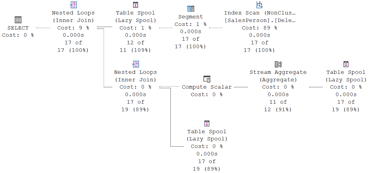
And this is the execution plan that I showed and explained in that post, and that you will still get for the above query in every version of SQL Server that I know of:
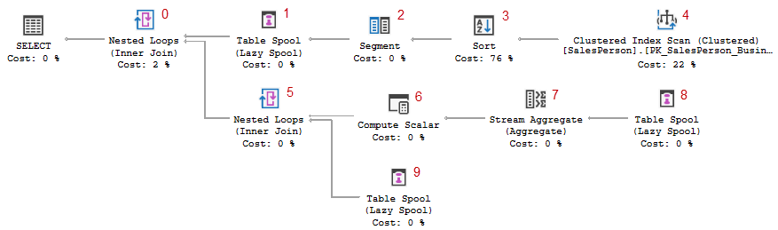
This post is from 2018. At that time, Management Studio did not yet include the estimated and actual number of rows in the execution plan with run-time statistics, which is why the oddities that I am going to focus on today were not very visible. So here is a new screenshot of the execution plan with run-time statistics for the same query, but now from Management Studio 22.9.2. Again with Node ID values added for easy reference.
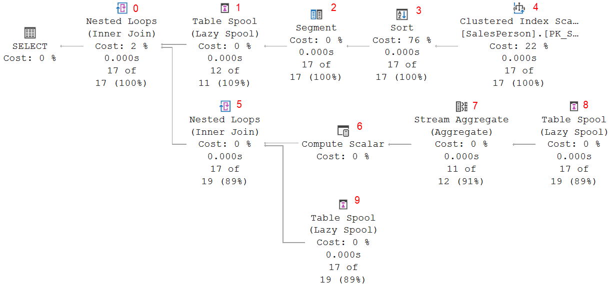
As you can see, Table Spool #1 is estimated to return 11 rows, but actually returns 12. But it is not the difference between estimated and actual that triggers me here. It is just the value of the Actual Number of All Rows property of this Table Spool. Why is this 12?
In my original post, I explained that a Table Spool that receives its input from a Segment operator will not return all rows it receives and stores in its worktable, but only return a single row for each segment. The Segment operator basically implements the PARTITION BY part of the query, by starting a new segment for each TerritoryID value. It is easy to see that the data has 11 such values: NULL (which counts as a value for this purpose, because all rows with a NULL here count as one partition for the window aggregate); plus each of the values 1 to 10. So that means that this Table Spool is supposed to return 11 rows, not 12. Where does this extra row come from and why is it there?
Segmented Table Spool bugged?
Let me first admit that I do not have a definitive answer here. But I do have a theory, plus some evidence to back it.
I believe that the code for a Table Spool running on segmented input data has a bug. Or perhaps glitch is a better word, because it does not cause harm anywhere. Except, as we have seen, in some unexpected values for its own Actual Number of Rows property, and for the Actual Number of Executions property of some other operators in the execution plan.
As I explained in plansplaining part 6, Table Spool #1 collects all rows from a segment, then returns a single row to represent that segment, which triggers the rest of the execution plan to create the results for that segment, using Table Spool #8 and #9 to read the data that Table Spool #1 has stored: all rows for the current segment.
But how does Table Spool #1 know when it has read the last row of a segment? It can only find out in one way: by calling its child operator, Segment #2, and receiving either a row with its segment column set, or the end of data signal. In the former case, we just hit the start of a new segment, so Table Spool #1 has to temporarily set this row aside in its operator memory (it can’t store it in the worktable yet, as that would make the row visible to Table Spool #8 and #9!), then return its single row, and wait until Nested Loops #0, or rather its bottom input, has finished processing the current segment. Once that is done, Nested Loops #0 will call Table Spool #1 again, which will now truncate the worktable, store the row from its operator memory in it, and then continue reading its input. And in the latter case, we moved past the end of the last segment, so we now only store the end of data marker in operator memory, return a row to Nested Loops #0, and when called again return that end of data marker so that execution can finish.
My suspicion is that the glitch in Table Spool is in how it processes the very first row. As the first row of a segment, it has its segment column set to True. Normally, that means the previous segment is now complete and has to be processed. But this is a special case. There is no previous segment. So Table Spool should just store this row and read the next.
I believe Microsoft forgot to code this exception. So what actually happens when Table Spool reads its first row is that it sets this row aside, and then returns a row to represent the (non-existing!!) previous segment.
The effect of this bug
 Nested Loops #1 receives a row, to represent the non-existing “segment zero”. It calls its child input, which starts (following the data) with Table Spool #8 reading from the worktable of Table Spool #1. This is empty, so Table Spool #8 instantly receives end of data. It returns this to Stream Aggregate #7. The properties of this Stream Aggregate do not include the Group By property, which means it does a scalar aggregation. Based on the query, you might have expected to see aggregation by TerritoryID. But remember, Table Spool #1, running in its special segmented mode, guarantees that Table Spool #8 only returns rows from a single segment, hence a single TerritoryID. So including or not including this Group By property makes no difference in this case. At least, not in the regular, non-glitched operation.
However, there is an important behavior difference between a scalar and a regular aggregate when their input is empty. For a regular aggregate, it means there are no groups, so nothing is returned. For a scalar aggregate, one row is returned, with 0 as the count (when requested), and NULL for all other requested aggregate functions. You can see this difference by running the sample query below:
SELECT   SUM (SalesYTD)
FROM     Sales.SalesPerson
WHERE    1 = 2
GROUP BY TerritoryID;

SELECT SUM (SalesYTD)
FROM   Sales.SalesPerson
WHERE  1 = 2;
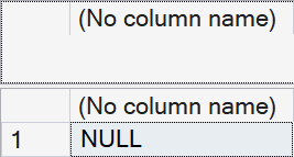
We already established that Stream Aggregate #7 uses scalar aggregation, so we now return a single row to Nested Loops #5, with a count (Expr1003) of 0 and the sum (Expr1004) set to NULL.
Nested Loops #5 now calls its bottom input. Table Spool #9 reads from the empty worktable that Table Spool #1 created and instantly returns end of data. The Logical Operation of Nested Loops #5 is Inner Join, so the row from Stream Aggregate #7 (and Compute Scalar #6) is not matched. Nested Loops #5 returns end of data to Nested Loops #0, which then also can’t return a match. And so it requests the next row from Table Spool #1, at which point actual processing of the first segment starts.
So no harm done. Just some cycles wasted, and some confusing counters in the execution plan that annoy geeks like me and are probably unnoticed by anyone else. Except that, even when it’s just a few cycles, it’s still wasted performance. And if this query runs a million times per day, it still adds up.
Trust, but verify
I don’t think it’s possible to know with 100% certainty whether my theory is completely correct. At least not without source code access. But with some creativity, it is definitely possible to see some things that make the theory more plausible.
I want to use the Live Execution Plan option (aka Live Query Statistics) to look in detail at what happens during each step of the process. However, the query finishes way too fast. So I have to be creative and build my own debugger. Not one that runs one query at a time, but one that allows me to process this query one row at a time.
For that purpose, I use row locks. If the third row that the execution plan reads is locked, then execution will pause after processing the first two. If I then also lock the fourth row, and then release the lock on row number three, I can then look at the Live Execution Plan to see exactly what happened during processing of that third row. Cumbersome, but effective.
This does require two things. First, we need to get rid of the Sort. Otherwise, locking a row will only delay when the Sort finishes and returns all data, and the rest of the plan still finishes near instantaneous. And second, we need to make sure that locks actually cause the query to block, so we can’t have snapshot or read committed snapshot isolation enabled.
So let’s first do these preparations:
ALTER DATABASE AdventureWorks2025
SET READ_COMMITTED_SNAPSHOT OFF WITH ROLLBACK IMMEDIATE;
ALTER DATABASE AdventureWorks2025
SET ALLOW_SNAPSHOT_ISOLATION OFF;
-- Supporting index
CREATE INDEX DeleteMeLater
ON Sales.SalesPerson (TerritoryID)
INCLUDE (SalesYTD);
The execution plan of the query now uses an ordered scan on the supporting index I created. The order of the query results matches the order of the input – which will become important when we want to lock just the right row.
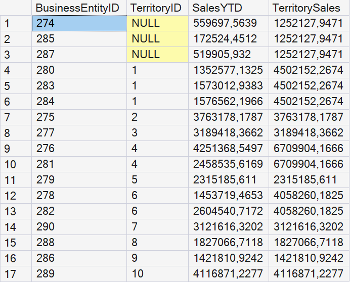
The preparations are done, so now the fun starts. First, I want to lock the first row, with BusinessEntityID 274. Since the query now uses the nonclustered index, I must ensure that at least one of the columns in this index is affected – else only the clustered index would be locked and the query would not wait. So let’s take the easy option and just modify the SalesYTD value:
BEGIN TRAN;
UPDATE Sales.SalesPerson
SET    SalesYTD += 1
WHERE  BusinessEntityID = 274;
--ROLLBACK TRAN;
Execute this, and make sure to leave the transaction open. We’ll roll it back later.
Now go back to the original query, enable the “Include Live Query Statistics” option, and then hit execute. The query will start, but the Index Scan is blocked when it tries to read the first row already. You should see this live execution plan:
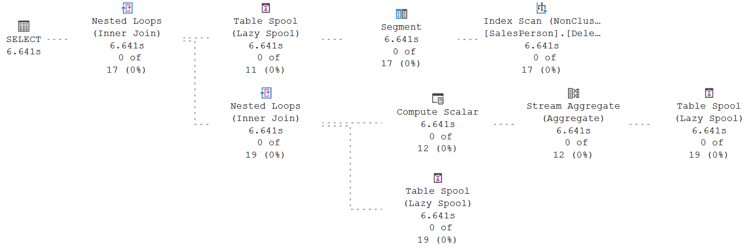
Index Scan has not returned any row yet. And that obviously means none of the other operators have returned anything yet. They have not even received anything to work on!
But more interesting is the Number of Executions property of each operator. You can’t see that in the screenshot above, but you can see it if you hover each of the operators. You will see that the entire top line lists a value of 1. Which is correct: this number is counted when an execution starts, and these operators have all been called. But the operators on the two bottom lines have not been called yet. And indeed, they all report their Number of Executions as zero.
We now want to process the first row. If you roll back the update above, that will happen, but the query will then instantly go on to process all other rows, and execution will be finished before you can even blink your eye. So we now need to first lock the second row, by opening yet another query window where we execute the query below:
BEGIN TRAN;
UPDATE Sales.SalesPerson
SET    SalesYTD += 1
WHERE  BusinessEntityID = 285;
--ROLLBACK TRAN;
Indeed. Exactly, the same, except the BusinessEntityID value is different. Not surprising. Once you have executed this query, both the first and the second row are locked.
You can now rollback the update on BusinessEntityID 274, simply by highlighting and executing the commented ROLLBACK TRAN statement. This releases the lock, and the SELECT query can now process this row. But as soon as the Index Scan tries to read the next row, execution will pause again. It does not matter that the lock was taken after the query started. Locking does not work based on when something was started, but only on the current situation. And that situation is that now, this row is locked for an UPDATE.
This is what the live execution plan now shows:
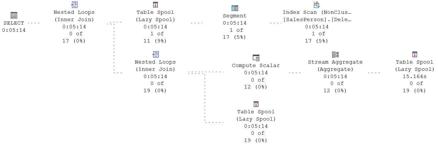
As you can see, the operators on the top row all returned 1 row now. That is the first row that we just allowed the Index Scan to read and return. Segment processes and passes it, Table Spool then stores it. But why did it also return a row? And why do the operators on the bottom input of the first Nested Loops now show their Number of Executions as 1? This can’t be explained by the “correct” behavior of a segmented Table Spool. But the bug that I described above explains it almost to a tee! Instantly after receiving its very first row, the segmented Table Spool returned a row, which caused the lower input of the Nested Loops to execute, but not produce any rows.
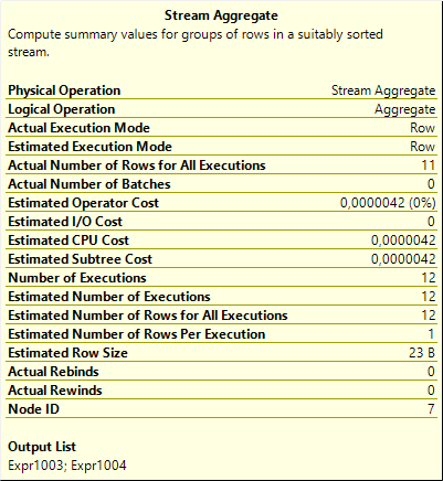
Almost? Yes, almost. There are three observations that do not match the expectation. Stream Aggregate should have returned this aforementioned row with NULL as the sum and 0 as the count, but the screenshot above shows zero rows returned. As a direct result of that Compute Scalar also shows 0 instead of 1. And that in turn results in the bottom Table Spool having a count of 0 instead of the expected 1. So three numbers that are different from my prediction, but they seem to have a common cause.
However, we’re doing science. When reality does not match a prediction, the theory has to be rejected. Well, unless we can find an explanation for the deviation. We’ll come back to this in a bit.
If you want to (I won’t describe it in detail here), you can keep stepping through the process using the same method. Modify the BusinessEntityID value in the update window that has no open transaction to put a lock on the next intended breakpoint, run it, then (and only then!) release the previous lock, and then look at the numbers in the live execution plan again. If you do, you will see that everything else is a perfect match for the behavior I predicted for a segmented Table Spool, including the “0th segment” glitch.
It still doesn’t all add up
I presented an explanation for the extra row returned by Table Spool, and the accompanying extra execution of Nested Loop #0’s bottom input. I also showed an experiment that at least confirms that this extra row and extra execution happen at the exact time predicted by my explanation. But we ran into a new problem. Stream Aggregate did not return the expected extra row, which also caused the number of executions of the bottom Table Spool to be one less than I had predicted.
I think I can explain that. But before I do, we need to do a sidestep into something completely different. Bear with me. This will become relevant.
The disappearing property
When a property in an execution plan can occur zero or more times, it is represented in the execution plan XML by nesting one or more instances of a property within a parent (container) property. A simple example can be seen in this very simple query, which uses the Constant Scan operator to return two rows with two columns each:
SELECT 1, 2
UNION ALL
SELECT 3, 4;
If you request the execution plan for this query and then open the execution plan XML, you will see that the rows and values to be returned are encoded as follows:
<ConstantScan>
  <Values>
    <Row>
      <ScalarOperator ScalarString="(1)">
        <Const ConstValue="(1)" />
      </ScalarOperator>
      <ScalarOperator ScalarString="(2)">
        <Const ConstValue="(2)" />
      </ScalarOperator>
    </Row>
    <Row>
      <ScalarOperator ScalarString="(3)">
        <Const ConstValue="(3)" />
      </ScalarOperator>
      <ScalarOperator ScalarString="(4)">
        <Const ConstValue="(4)" />
      </ScalarOperator>
    </Row>
  </Values>
</ConstantScan>
As you can see, <ConstantScan> has just one <Values> node, which in this case contains two <Row> nodes, each of which in turn contain two <ScalarOperator> nodes. Modify the query to add or remove columns or rows, and the number of corresponding elements will change.
You may have noticed an oddity in the first sentence of this section. I wrote about properties that occur “zero or more” times, yet I said that these are represented by nesting “one or more” instances of the property. This is not a mistake. At least, not by me. To illustrate this, let’s look at this simple sample query:
SELECT     abv.[Database Version],
           abv.VersionDate
FROM       dbo.AWBuildVersion AS abv
CROSS JOIN (SELECT 1, 2
            UNION ALL
            SELECT 3, 4) AS m(a, b);
The same query as before is now used as a subquery, with a CROSS JOIN to another table. But it is relevant to note that columns m.a and m.b are not used in the query. The optimizer knows this, so it won’t generate them. It still needs to generate two rows, though. These rows now have zero columns each. Not something we can do (I can remove one of the columns from the query above but nt both). But not a problem for the internal execution plan.
So in the execution plan XML, you now probably expect to see this fragment:
<ConstantScan>
  <Values>
    <Row>
    </Row>
    <Row>
    </Row>
  </Values>
</ConstantScan>
Or perhaps this alternative representation:
<ConstantScan>
  <Values>
    <Row />
    <Row />
  </Values>
</ConstantScan>
But that is not the case! Here is what the relevant fragment of the execution plan XML actually looks like:
<ConstantScan />
Yeah. That is right. All the <Row> elements have disappeared, and so has the <Values> element. The result is that the <ConstantScan> element is now empty.
The reason is a shortcoming in the code that exports the internal representation of the execution plan into the XML format. In several cases, such as this, it doesn’t handle empty collections well. So if there are zero columns and hence zero <ScalarOperator> elements, then, instead of returning an empty <Row> element, it just omits the <Row> element completely. Which then makes the <Values> element empty, and that then also gets omitted from the execution plan XML. So if you change the sample query to have one, three, or forty-two rows, the execution plan XML (and hence also the graphical execution plan) remain fully unchanged. I don’t know of any way to access the internal representation of the execution plan, but if there is any, then that is the only place where you would see how many of these empty rows Compute Scalar will return.
The scalar aggregate that isn’t a scalar aggregate
So let’s now return to our Stream Aggregate. I previously wrote that it changes from regular aggregation to scalar aggregation if there is no Group By property. And we saw no Group By property, so the logical conclusion was: scalar aggregation. But it is important to know that the Group By property is represented in the execution plan XML as a <GroupBy> element that contains one or more nested <ColumnReference> elements. Which makes sense. After all, a GROUP BY can list more than one column or expression, such as in the following sample query:
SELECT   sp.TerritoryID,
         sp.CommissionPct,
         SUM (sp.SalesYTD) AS TerritorySales
FROM     Sales.SalesPerson AS sp
GROUP BY sp.TerritoryID,
         sp.CommissionPct;
In the execution plan XML, we now find this fragment (lines might wrap):
<GroupBy>
  <ColumnReference Database="[AdventureWorks2025]" Schema="[Sales]" Table="[SalesPerson]" Alias="[sp]" Column="CommissionPct" />
  <ColumnReference Database="[AdventureWorks2025]" Schema="[Sales]" Table="[SalesPerson]" Alias="[sp]" Column="TerritoryID" />
</GroupBy>
I just showed that there are cases where a repeated element that can have zero occurrences in the internal execution plan is simply omitted from the execution plan XML in such a case. What if the <GroupBy> element of a Stream Aggregate is also such an example? In that case, the internal execution plan could distinguish between not having a <GroupBy> at all (for scalar aggregation), or a <GroupBy> with zero <ColumnReference> elements (for regular aggregation over an empty column list). And while the two behave exactly the same as long as there is data to aggregate, there is a difference when the input is empty. Scalar aggregateion is defined to always return exactly one row, even when the input is empty. Regular aggregation is defined to return one row for each group in the input. On empty input, there are no groups, so no results.
So this is my theory. Stream Aggregate #7 (in the original plan, after removing the Sort its Node ID changed to 6) looks like a scalar aggregate to us, because we do not see any Group By property. But that is the result of a glitch in the export of the internal execution plan to the XML representation that we get to see. The internal version of the execution plan does have a <GroupBy> element, but it’s empty. So we don’t do scalar aggregation; we do regular aggregation on the empty set.
And while I can’t prove this in any way, because I do not know any way to access the internal version of the execution plan, it does explain exactly the small mismatch we had before. Now I understand why, after processing the first row, Stream Aggregate did have an execution, but did not return any rows – it did a regular aggregation, not a scalar aggregation, on its empty input, which makes no rows the correct results. And this then also explains why Compute Scalar returned no row either, and why the bottom Table Spool did not execute at that time.
Conclusion
An explanation on an execution plan can only be correct when every detail fits. That was not the case with my original explanation for the execution plan for frameless window aggregates, as presented in plansplaining part 6. This post fixed that.
I first explained how Table Spool acts on a frame change and posited that it incorrectly also does these actions for the (nonexisting) “0th segment” when it receives its first row. While I can’t prove this, an experiment where I make the query process one row at a time does make it seem very plausible.
However, this explanation could not explain all oddities. To fix that, I then also posited that a Stream Aggregate can have an empty Group By property, but this is not visible in the graphical or XML representations of the execution plan. Again, impossible to prove, but made more likely by looking at a similar situation in another operator that does not show certain properties when their content is an empty list.
As always, this series is for the reader. If you have ever encountered an execution plan where you could not quite work out how everything fit together, let me know. I will be happy to investigate it, and then describe all the details in a future post.